Article citation information:
Rzydzik,
S., Panfil, W., Myszor, D., Cyran, K., Moczulski, W. Improvement
of the agility and manageability of an autonomous blimp. Scientific Journal of Silesian University of Technology. Series
Transport. 2026, 131, 189-205. ISSN:
0209-3324. DOI: https://doi.org/10.20858/sjsutst.2026.131.12
Sebastian RZYDZIK[1],
Wawrzyniec PANFIL[2],
Dariusz MYSZOR[3],
Krzysztof CYRAN[4],
Wojciech MOCZULSKI[5]
IMPROVEMENT OF THE AGILITY AND MANAGEABILITY OF
AN AUTONOMOUS BLIMP
Summary. This paper presents the development and experimental
validation of a control-oriented numerical model and a PID-based autonomous
control system for an unmanned blimp. A simplified dynamic model was
implemented in the GNU Octave environment and used for the systematic tuning of
vertical and horizontal propulsion controllers. Experimental identification
using a full-scale blimp prototype demonstrated good agreement between
simulated and real flight responses, with mean time errors below 5% and
altitude errors below 1% in representative vertical maneuvering
experiments. Indoor flight tests performed with a Pixhawk autopilot confirmed
stable autonomous altitude control, with steady-state altitude deviations
limited to approximately 4-5 cm, as well as reliable target-point acquisition
during autonomous navigation. The results demonstrate that the proposed
numerical model enables fast and effective controller tuning while maintaining
sufficient accuracy for real-world implementation and that the tuned PID controllers
provide stable, smooth, and repeatable autonomous flight suitable for
inspection and monitoring applications.
Keywords: inspection
and monitoring, autonomous airship, control system, virtual teleportation
1. INTRODUCTION
There
is a growing trend of using unmanned aerial vehicles (UAVs) for sustained
inspection and monitoring operations. Illustrative examples include the
surveillance of sporting events, such as football matches; large-scale cultural
events, such as outdoor concerts; and the inspection of expansive
infrastructure, such as railway lines and highways. In such scenarios, where
UAVs are often limited by constrained energy resources, contemporary airships
are poised to assume an increasingly significant role. Recognizing this
potential, the SkyTech Products Research and
Development team has launched a research initiative with the objective of
developing a ground-based remote-control station for UAVs, with airships
representing a primary category.
A
review of the existing literature indicates that while advanced airship control
strategies and high‑fidelity dynamic models have been widely
investigated, there remains a practical need for control‑oriented
numerical models that support the implementation and tuning of classical
controllers in real aerial blimps. In particular, despite the widespread use of
PID control in airship applications, the criteria and conditions for its tuning
are often not explicitly discussed.
Therefore,
the objective of this paper is to develop a simplified numerical model of an
unmanned airship suitable for control design and to implement and tune PID
controllers for vertical and horizontal propulsion systems. The proposed
approach focuses on achieving stable and reliable maneuvering
behavior under representative operating conditions.
This
paper presents the development process of a dedicated autopilot algorithm and
its implementation in software specially geared to aerial blimps. It is
composed as follows: Section 3 describes a numerical model, which is
further implemented in the GNU Octave simulation environment. Section 4 shows
an implementation of the control algorithms on a real unmanned airship. To this
end, a well-known PixHawk autopilot module has been
implemented. The next section deals with exhaustive experiments whose goal has
been to estimate and tune different parameters of the developed model. Several
scenarios have been proposed, and then proper experiments were carried out
whose results were analyzed to yield basic statistics
characterizing inherent data deviation. Then, in Section 6, an experimental
verification of the control algorithms is shown. The article ends with
conclusions.
2. LITERATURE REVIEW
The
field of aviation, long dominated by fixed-wing aircraft and rotary-wing
helicopters, is witnessing the resurgence of a unique aerial platform: the
airship [8, 1]. These lighter-than-air vehicles, buoyed by gases such as
helium, possess inherent advantages that are driving renewed interest in their
development and deployment. Unlike heavier-than-air platforms, airships excel
in endurance, offering prolonged flight times and efficient hovering [12]. This
characteristic enables a wide range of applications, from persistent
surveillance and long-haul cargo transport to indoor inspections and
entertainment robotics [4, 5]. However, the interaction of airships with
aerodynamic forces and the challenge of achieving precise control introduce
significant engineering difficulties that require advanced solutions [13].
This
review of airship control systems reveals a field combining established
principles with modern innovations. The fundamental challenge lies in
effectively governing airship motion, enabling navigation in three-dimensional
space, maintaining orientations, and executing complex maneuvers
with accuracy and reliability [1, 8]. Meeting these requirements demands a
thorough understanding of airship dynamics, acting forces, and robust control
algorithms capable of translating commands into precise actuator responses.
A
major difficulty in airship control arises from their inherent underactuation. In contrast to multirotor drones that can
control all degrees of freedom independently, airships typically have fewer
control inputs than controlled motions [13]. As a result, certain movements are
coupled and cannot be controlled directly; for example, lateral motion often
requires prior rotation. This characteristic increases control complexity and
necessitates advanced strategies to ensure stability and performance.
Environmental
disturbances further complicate control tasks. Due to their large surface area,
airships are highly sensitive to wind effects, including gusts and turbulence,
which can significantly disrupt motion and trajectory tracking [8, 9, 13].
Consequently, control systems must be robust and adaptive to maintain safe and
reliable operation under varying atmospheric conditions.
The
physical design of the airship also strongly affects controllability.
Parameters such as hull shape, size, and mass distribution directly influence
dynamic behavior [4, 12]. Research has examined
various geometries to balance aerodynamic efficiency and maneuverability,
with studies highlighting the role of the slenderness ratio in stability and
performance [12]. Alternative configurations, including spherical blimps
equipped with tetrahedrally arranged thrusters, have been proposed to enhance
agility and enable omnidirectional motion [4].
Application-driven
research continues to expand. Indoors, compact and highly maneuverable
airships are considered for tasks requiring safe operation near obstacles or
humans, such as confined-space inspections, vertical farm monitoring, and
interactive entertainment [5, 12]. Emphasis is placed on precise low-speed
motion, stable hovering, and collision avoidance. The BlimpleBee
platform exemplifies this development trend, demonstrating the feasibility of
helium-assisted vehicles for delicate inspection missions [4].
For
outdoor missions, priorities shift toward endurance, payload capacity, and
robustness to weather disturbances. Autonomous airships are envisioned for
long-term surveillance, environmental monitoring, and cargo transport, offering
efficiency advantages over conventional drones [8, 12]. These applications
impose stringent requirements on control systems, including disturbance
rejection, long-range navigation, and reliable stability.
Safety
and reliability are particularly critical when airships operate near people or
in hazardous environments, such as disaster response scenarios [4]. Hybrid
platforms that combine lighter-than-air properties with multirotor redundancy,
such as the Janus system, address these concerns by enabling fallback flight
modes in case of buoyancy failure [11].
To
tackle the diverse challenges of airship control, researchers have explored a
broad range of methodologies. Classical approaches, including PID control,
remain widely used due to their simplicity and effectiveness for basic
stabilization tasks [1, 8]. Nonetheless, their limitations in nonlinear and
uncertain environments have motivated the adoption of advanced strategies.
Adaptive
control allows online parameter adjustment to compensate for model
uncertainties, while robust control methods guarantee stability under bounded
disturbances [13]. Model Predictive Control (MPC) exploits future-state
predictions to optimize control actions, and intelligent approaches, such as
reinforcement learning, are increasingly investigated to enable learning-based
adaptation to complex environments [8].
Accurate
dynamic modeling is a prerequisite for controller
development and validation. This involves capturing buoyancy, aerodynamic
forces, and in some cases tether interactions [1, 9]. Mathematical models
derived from stability derivatives and computational fluid dynamics (CFD)
analyses are commonly used for simulation-based controller design [12].
Despite
extensive research on airship aerodynamics and advanced control strategies,
fewer studies address the practical implementation and tuning of classical
controllers based on control-oriented numerical models. In particular,
systematic procedures for selecting PID gains in underactuated airship systems
remain insufficiently documented.
Motivated
by this gap, the present study focuses on developing a numerical model suitable
for closed-loop simulations and investigating the implementation and tuning of
PID controllers for vertical and horizontal motion control of an unmanned
airship.
3. NUMERICAL MODEL
3.1. Mathematical model
The
development of the numerical model began with an analysis of existing
mathematical models of blimps, including both kinematic and dynamic
formulations. A brief overview of the adopted modeling
assumptions is presented below.
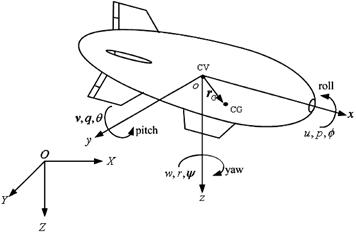
Fig. 1. Reference frames and motion parameters
of the blimp [14]
Based
on the reference frames shown in Fig. 1, the inertial coordinate system is
defined as follows: the x-axis points to True North, the y-axis
points east, and the z-axis points downward. The linear velocity
components in the body-fixed frame are denoted by u (longitudinal), v (lateral),
and w (vertical). The Euler angles are defined as θ (pitch), ϕ (roll), and ψ (yaw), while the angular velocity
components are denoted by p, q, and r, corresponding to
roll, pitch, and yaw rates, respectively.
The
kinematic equations of motion of the blimp can be expressed as
 (1)
(1)
Where:

is the
position vector in the inertial frame,

is the
linear velocity vector expressed in the body-fixed frame,

is the
vector of Euler angles, and

is the
angular velocity vector. The matrices  and
and  represent the rotation matrix and the kinematic
transformation matrix, respectively.
represent the rotation matrix and the kinematic
transformation matrix, respectively.
The
dynamic behavior of the airship is described using
the Newton-Euler formalism
 (2)
(2)
 (3)
(3)
where F
and τ
denote the resultant external forces and moments acting on the vehicle,
including aerodynamic forces, buoyancy, gravity, and propulsive thrust. The
vector
 (4)
(4)
represents
the displacement of the center of gravity (CG)
relative to the center of volume (CV). The inertia
tensor with respect to the origin of the body‑fixed frame is defined as
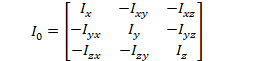 (5)
(5)
with the
symmetry conditions  ,
,  , and
, and  .
.
The
mass m in Eqs. (2)-(3) denotes the total
effective mass of the airship, including the envelope, gondola, propulsion
system, and payload.
The
total mass and inertia were modeled as sums of rigid‑body
and added‑mass contributions

where  and
and  are the
rigid‑body mass and inertia tensor, while
are the
rigid‑body mass and inertia tensor, while  and
and  represent the added mass and added inertia
arising from the acceleration of the surrounding air.
represent the added mass and added inertia
arising from the acceleration of the surrounding air.
The
added‑mass terms were estimated using an ellipsoidal approximation of the
airship envelope. The hull was approximated as a prolate spheroid whose
principal axes correspond to the longitudinal and transversal dimensions of the
envelope. Under the assumption of inviscid potential flow, the added mass and
added inertia coefficients were determined as functions of the airship geometry
and the displaced air volume.
The
added‑mass and added‑inertia contributions were incorporated
directly into the effective mass and inertia terms in Eqs.
(2)-(5). This formulation is well suited for maneuvering
simulations and ensures a physically consistent representation of translational
and rotational fluid-structure interaction effects.
Further
details of the mathematical background and parameter estimation methods can be
found in [2, 6, 7, 10, 14].
The
main objective of this study was the implementation and tuning of PID
controllers for the vertical and horizontal propulsion systems. For vertical
motion control, the following control law was applied:
 (6)
(6)
where
 is the vertical thrust ratio,
  is the
altitude error,
is the
altitude error,  is the vertical velocity, and
  ,
,  , and
, and  are the
proportional, integral, and derivative gains, respectively.
are the
proportional, integral, and derivative gains, respectively.
Yaw
motion was controlled by differential thrust of the horizontal propellers
 (7)
(7)
 (8)
(8)
where  and
and  denote the right and left thrust ratios,
  is the
yaw angle error,
is the
yaw angle error,  is the
yaw rate, and
is the
yaw rate, and  ,
,  , and
, and  are the
controller gains.
are the
controller gains.
3.2. Implementation of the blimp numerical
model
The
numerical model incorporates the following elements:
- geometric
properties, such as longitudinal and transversal cross-section dimensions;
- mass
properties, including mass distribution and moments of inertia;
- thruster
characteristics, specifically thrust generation;
- aerodynamic
properties, such as drag coefficients;
- external
disturbances, including wind direction and speed.
The
aerodynamic forces were modeled using a simplified
quasi‑static formulation. The drag forces along the principal body axes
were assumed to be proportional to the corresponding velocity components. Lift
and side‑force effects were neglected due to the low operating speeds and
small angles of attack considered in the simulations. This level of modeling detail was found sufficient for control design and
performance evaluation purposes.
The
model was developed based on the approaches described in [2, 3] and implemented
using the ode45 solver. With appropriate solver configuration, the model
generates time histories of key state variables, including spatial position,
Euler angles (yaw and pitch), thrust commands for vertical and horizontal
propellers (left and right), linear velocities, and angular velocities.
The
PID controller parameters were selected based on closed‑loop simulation
studies. The tuning criteria included stability of the airship motion,
acceptable settling time, limited overshoot in altitude and yaw responses, and
smooth actuator commands within admissible thrust limits. The parameters were
adjusted under representative operating conditions relevant to low‑speed maneuvering tasks.
Simulation
results obtained using the numerical model are presented in the second part of
this paper.
4. INTEGRATION OF THE BLIMP CONTROL MODEL WITH
PIXHAWK AUTOPILOT
4.1. Geometrical properties of the blimp
prototype
Figure 2 shows the physical blimp prototype
used in this study, while Figure 1 presents a schematic
representation of the adopted reference frames and motion parameters.
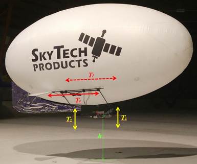
Fig. 2. The blimp prototype: Tr
– right horizontal thrust, Tl – left horizontal thrust,
Tz – vertical thrust
The geometry of the airship envelope was
approximated using an ellipsoidal model, consistent with the schematic
representation shown in Fig. 1. The hull can be described as
a prolate spheroid with semi‑axes  ,
,  , and
, and  , where corresponds to the
longitudinal axis and
, where corresponds to the
longitudinal axis and  to the transversal
axes. For the prototype used in this study, the overall length of
the envelope was approximately
to the transversal
axes. For the prototype used in this study, the overall length of
the envelope was approximately  , while its maximum
diameter was approximately
, while its maximum
diameter was approximately  . This corresponds to
semi‑axes
. This corresponds to
semi‑axes  and
and  , yielding
a slenderness ratio
, yielding
a slenderness ratio  .
.
These geometric parameters were used to estimate the
displaced air volume and to determine the added‑mass and added‑inertia
coefficients employed in the numerical model. The ellipsoidal approximation
provides a reasonable balance between physical accuracy and computational
simplicity and is commonly adopted in control‑oriented modeling of airships.
The stabilizing surfaces visible in Fig. 1
represent simplified tail fins intended primarily to enhance passive
directional stability. Due to their small size and integration with the
envelope, these surfaces are not clearly distinguishable in the photograph of
the prototype shown in Fig. 2. In the current configuration, active
control authority is provided exclusively by the vertical and horizontal
propellers, while the stabilizing surfaces contribute only to passive
aerodynamic damping and static stability effects, which are implicitly
represented in the simplified aerodynamic model.
4.2. The idea of autonomous control
Figure
3 presents the conceptual architecture of the autonomous control system
implemented for the blimp.
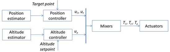
Fig.
3. Idea of an autonomous control system
The
control of the flight consists of two independent control loops:
1)
Vertical movement control – the height of
the blimp above the ground (altitude) is continuously controlled by vertical
thrust (Tz) and based on:
a)
altitude error calculated from the
measurement of distance to the ground (h) using a laser distance sensor
mounted on the bottom of the nacelle;
b)
vertical speed obtained by numerical
differentiation of the altitude measurement (h) or directly from the IMU
in the Pixhawk.
2)
Horizontal movement control – the
horizontal position of the blimp is continuously controlled by the left (Tl)
and right (Tr) thrusts and based on the following:
a)
horizontal position error calculated from
the actual GPS data and target point;
b)
angle error calculated from the compass
data, actual and target point;
c)
yaw rate calculated from the gyroscope
data – however, this information is not used at this stage and will be
incorporated in future work.
4.3. Autonomous flight controller
The
blimp control system was implemented using a Pixhawk flight controller. A
dedicated module, named blimp_control, was
developed in accordance with the PX4 Development Guide.
In
the standard PX4 Airship configuration, thrust vectoring is handled
within the mixer, allowing tilting actuators to simultaneously affect multiple
motion axes. This results in a coupled control structure. In contrast, the
proposed control system is tailored to the specific blimp configuration and
employs a decoupled approach: two fixed horizontal propellers generate forward
motion and yaw through differential thrust, while dedicated vertical propellers
independently regulate altitude. This separation simplifies the control design and
improves the transparency of the control structure.
The blimp_control module:
1)
implements a PID controller for vertical
motion (altitude) control;
2)
implements a simplified rule‑based
controller for horizontal motion and navigation. A PID‑based controller,
previously developed and validated in numerical simulations (see
Section 3), is planned to be implemented in future work.
The blimp_control module uses a set of configurable
parameters that can be adjusted in real--time using QGroundControl
via the MAVLink communication protocol, without the
need to reprogram or restart the autopilot.
5. EXPERIMENTS FOR TUNING MODEL PARAMETERS
The
identification of the blimp parameters consisted of:
1)
Development of experiments scenarios.
2)
Conduct experiments using the physical
blimp model.
3)
Analysis of the measurement results.
4)
The choice of the parameter values for the
mathematical model.
5.1. Scenarios of experiments
The
purpose of the development of scenarios was to measure the response of the
parameter values of the physical blimp model to known values of external
impacts. The description of one of four example scenarios is presented below.
Tab.
1
Scenario example
|
Name |
Changing the vertical thrust to the
opposite |
|
Stages |
1. Place the blimp at a height of about 1 m. 2. Free the blimp and simultaneously run the
vertical thrust fan (VFan) at 20% for 8 s. 3. Then, after 8 s from the beginning of the
experiment, run the vertical thrust fan (VFan) at
-20% for 4 s. 4. Leave the blimp until it falls to ground
level. |
|
Expected behavior |
1. The blimp should lower its initial
height. 2. Then, the blimp should increase its
height, even after turning off the fan of the vertical thrust. 3. After the reverse vertical thrust is
turned on, the blimp should quickly reduce its height (even when the fan is
turned off) until the ground level is reached. |
|
Observed features |
1. Maximum altitude measured from the
ground. 2. The time to climb to the maximum altitude
and the time to descend from the maximum altitude to the ground level. |
|
Comments |
If the expected behavior of the blimp is
not consistent with the description, it is possible to extend or shorten the
duration of the vertical thrust of the fan, or reduce the thrust. |
5.2. Results of experiments using the real
blimp model
The scenario described above was the basis for conducting experiments on the real model of a blimp. Each experiment was performed 10 times, and the obtained data were subjected to statistical analysis (see Tab. 2). The following features have been recorded:
·
horizontal and vertical thrust;
·
unbalance weight;
·
starting altitude;
·
maximum altitude;
·
time of positive and negative thrust;
·
time of climb; and
·
fall time.
Tab.
2
Summary of the statistical analysis of
experimental data
|
Vertical thrust [g] |
Unbalanced mass [g] |
Starting altitude [m] |
Maximum altitude [m] |
Duration of positive thrust [s] |
Climb time [s] |
Duration of negative thrust [s] |
Descent time [s] |
|
|
Average |
62,7 |
18,2 |
1 |
5,43 |
8,4 |
8,5 |
5,0 |
22,8 |
|
Std. deviation |
1,27 |
3,31 |
0 |
0,36 |
0,19 |
0,17 |
0,72 |
2,89 |
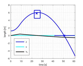
Fig.
4. The result of tuning the numerical model with the estimated error
5.3. Tuning of the blimp numerical model
The
aim of the numerical model tuning process was to adjust its parameters to the
values of the features measured during the experiments using the real blimp
model. The basic criterion was to minimize the time and distance errors for
each experiment, assuming the same values as the numerical model of the blimp.
The example of tuning characteristics, in the case of changing the vertical
thrust to the opposite, is shown in Fig. 4. In this experiment, the mean time error is equal to 4.84% (2.16[s]) and the mean
z-length error (height) is equal to -0.43% (0.024[m]).
5.4. Examples of simulations using the
controller numerical model
In
the case of the vertical thrust controller, the mission focused on maintaining
the flight altitude at 15-7.5-15 [m], with variable wind in the range <-1;
1> [m/s]. The results for the vertical thrust PID controller model with
"soft" settings, for  , have been shown in Fig. 5.
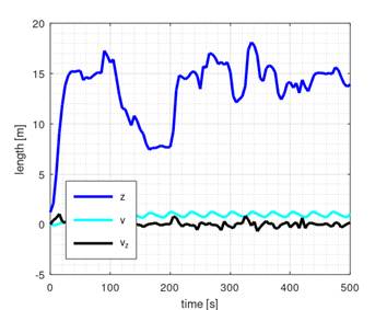
Fig.
5. The result of the numerical simulation: keeping altitude with wind
In
the case of the horizontal thruster controller, the purpose was to fly in
proximity of four points, defining a square under a side of 30 [m], with the
assumption of lack of wind. The results of this simulation are shown in Fig. 6.
The flight time was set at 500 [s]. PID parameters:  .
.
The
results of a similar mission as before, but in the case of variable wind in the
range
of <-1; 1> [m/s], are shown in Fig. 7.
6. EXPERIMENTAL VERIFICATION OF AUTONOMOUS
CONTROL OF
THE BLIMP
6.1. Balancing the blimp
During
the experiments, it was observed that the helium inside the envelope of the
blimp evaporates over time. In consequence, the blimp becomes unbalanced, i.e.,
overloaded. It is extremely important to keep the blimp well balanced when
developing altitude control algorithms. To do that, a bottle filled with salt
has loaded the blimp. The amount of salt was constantly monitored.
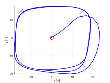
Fig.
6. The result of numerical simulation: flying in the proximity to four points
without wind
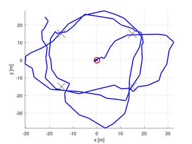
Fig.
7. The result of a numerical simulation: flying in proximity to four points
in windy conditions
6.2. Experiments leading to the development of
autonomous altitude control
Many
experiments were carried out that led to final development and implementation
of the elaborated (within numerical experiments, see Section 2) PID algorithm
for vertical autonomous control. All these experiments took place inside the
Ice Skating Hall of the Silesian University of Technology in Gliwice, Poland
(Fig. 8). Exemplary experiments are discussed below and are documented in
videos (available on the YouTube channel Blimp Experiments:
https://www.youtube.com/playlist?list=PL-0gX2KowkKvQRTEmx0E84VluRMJ6jUTW) – it
is recommended to enable audio playback when watching these videos.
The
exemplary experiments are as follows:
1) Autonomous
altitude control [video: 1_AutoHeight]
In
this experiment, the blimp hovers at a specified altitude, i.e., 1.25 [m]. The
following PID parameters were applied (Kpv
= 0.1, Kiv = 0.25, Kdv
= 0.8). These parameters were predetermined within numerical experiments.
Observations/conclusions:
When the blimp is well balanced, the vertical propellers almost do not work.
Over time, when the airship becomes increasingly unbalanced, the propellers
spin faster and faster.
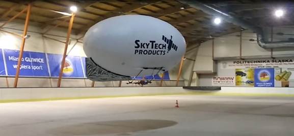
Fig. 8. Experimental verification of autonomous
control
2) Flying up
to the altitude setpoint [video: 2_AutoHeightFromBottom]
In
this experiment, the blimp is released below a desired altitude (1.25 [m]) and
flies up. Then it maintains the altitude. The same PID parameters as in
experiment 1.
Observations/conclusions: at the beginning, the blimp is underloaded and flies up to the desired altitude. We can observe that the propellers do not work even below the given altitude because the D part of the PID controller takes into account the vertical speed of the blimp. When the blimp is close to the given altitude, the controller tries to “defend” against excessive crossing of a given point – it was observed when the blimp both flies up and down. Then the blimp hovers very well.
3) Flying to
altitude setpoint [video: 3_AutoHeightFromTop]
In
this experiment, the blimp is released above the desired altitude (1.25 [m])
and flies down. Then it maintains the altitude. The same PID parameters as in
experiment 1.
Observations/conclusions: we can observe that at the beginning the propellers work very hard because the blimp is underloaded. Then the propellers stop working or even try to raise the blimp because the D part of the PID controller takes into account the vertical speed of the blimp - the controller tries to ‘defend’ against excessive crossing of a given point. Then the blimp hovers very well.
4) Autonomous
altitude control (with ‘mild’ PID parameters) [video: 4_AutoHeightMildPID]
In
this experiment, the blimp starts at 1.25 [m], then flies up to 2.25 [m] and
then flies back (down) to 1.25 [m]. The ‘softer’ PID parameters were applied (Kpv = 0.2, Kiv = 0.16, Kdv = 4.8 for downward or Kdv = 1.2 for upward movement) compared
to those of experiments 1-3. These parameters were predetermined within the
numerical experiments.
Observations/conclusions:
it can be seen that the blimp reaches the given altitude very smoothly and does
not cross a given point very much. Of course, the time necessary to reach the
given altitude is much longer compared to those from Experiments 2 and 3.
5) Autonomous
altitude control (with tape measurements) [video: 5_AutoHeightWithTape]
In
this experiment, the blimp hovers at a specified altitude and the vertical
position of it is measured. The same PID parameters as in experiment 1.
Observations/conclusions:
We can observe that the good balanced blimp is able to hover very well within
4-5 [cm].
6) Autonomous
flying up and down [video: 6_AutoHeight_125_225]
In
this experiment, the flies fly up and down between altitudes of 1.25 and 2.25
[m]. The same PID parameters as in experiment 1.
Observations/conclusions:
it was observed that the blimp is well balanced. It crosses the specified
altitudes, oscillates little and hovers quite well.
7) Manual
position control with autonomous altitude control [video:
7_AutoHeightManualDirection]
In
this experiment, the horizontal movement of the blimp is controlled manually by
the operator, but the given altitude is controlled simultaneously autonomously.
The same PID parameters as in experiment 1.
Observations/conclusions:
we can observe that the altitude is controlled autonomously quite well. Of
course, because of the more dynamic overall behavior
of the blimp, we can see that the blimp dives during turns, but it defends
itself against hitting the surface of ice rink.
6.3. Experimental verification of autonomous
movement of the blimp to the selected target point
When
the altitude controller was finished, then the position controller was
developed. To this end, the simplified rule-based controller was implemented
and verified. In the near future, the elaborated PID position controller (see
Section 1) will be implemented. For all of these experiments, a target point
was defined with coordinates: 50.2872338504249° (latitude), 18.6871733366383°
(longitude) – this is a center of the ice rink (see a
traffic bollard in Fig. 9).
The
exemplary experiments carried out so far are as follows:
1) Autonomous
flying to the target point without stopping at this point [video:
8_AutoHeightAutoThroughPoint]
In
this experiment, the altitude and position are controlled autonomously. The
blimp flies to the given target (center of ice rink
marked with a traffic bollard) and does not stop at this point.
Observations/conclusions:
When the blimp reaches the target point (within a dead zone of radius 3 [m]) it
stops the horizontal propellers and flies further due to its inertia. As
a consequence, it flies through the target and then turns back. This behavior repeats over and over again – the blimp loiters.
2)
10) Autonomous flying to target point with
a stop at this point (example 1, example 2) [videos: 9_AutoHeightAutoToPoint1,
10_AutoHeightAutoToPoint2]
3)
In this
experiment, the altitude and position are controlled autonomously. The blimp
flies to the given target (center of ice-rink marked
with traffic bollard) and stops at this point.
4)
Observations/conclusions:
we can observe that the blimp is able to reach the target point and
simultaneously maintain the altitude.
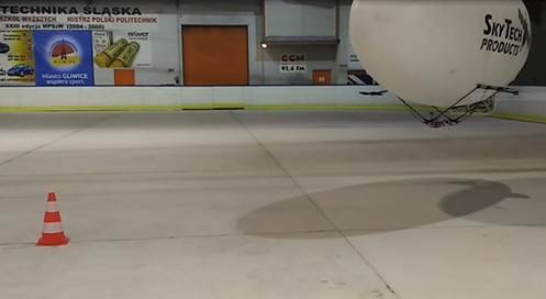
Fig. 9. Blimp reaching a target point (traffic
buoy located in the center of the ice rink)
7. CONCLUSIONS
The
experiments carried out provided valuable information on the behavior and control of an aerial blimp, leading to several
key conclusions. First, the data acquired from real-world experiments proved
crucial for accurately tuning the parameters of the developed numerical model
of the blimp. This alignment between the simulated and physical systems is
essential for reliable virtual testing and control strategy development.
Second, the use of this validated numerical model significantly reduced the
time and resources typically associated with the development and implementation
of a control strategy. By allowing for virtual experimentation and refinement,
the model simplified the overall process.
Observations
of the numerical model's responses to defined drive controller settings
demonstrated that the blimp's movement trajectories are predictable and the
quality of these responses was deemed satisfactory. This predictability is a
fundamental requirement for designing effective control algorithms.
Furthermore, the experiments highlighted the importance of proper balance to
maintain a consistent altitude. An imbalanced blimp requires continuous control
adjustments to counteract unwanted vertical movement.
Interestingly,
it was observed that even when subjected to disturbances causing rotation along
the pitch axis, the blimp could maintain its altitude. This inherent stability
in the vertical plane under pitch perturbations is a noteworthy characteristic.
The potential benefit of independently controlling vertical propellers was also
recognized, as this could mitigate unwanted rotation around the pitch axis,
leading to more stable and precise vertical control.
Currently,
the real blimp's position is managed by a straightforward rule-based
controller, which performs adequately. However, based on the promising results
obtained from numerical experiments with a PID
(Proportional-Integral-Derivative) controller, it is anticipated that
implementing this more sophisticated control algorithm on the physical blimp
will lead to even better performance, characterized by enhanced accuracy,
stability, and responsiveness in its movements. In summary, the research
underscores the value of numerical modeling in the
development of the airship control system and identifies key factors and
potential improvements to achieve precise and robust blimp control.
Acknowledgments
The
project was implemented in cooperation with SkyTech
Products sp. z o.o.
References
1.
Åman Gustaf. 2021. Indoor
Blimp Control. Master’s Thesis TFRT-6134. Lund, Sweden: Department of
Automatic Control, Lund University.
2.
Ashraf Muhammad Zahir, Mohammad A. Choudhry. 2013. „Dynamic Modeling of
the Airship with Matlab Using Geometrical Aerodynamic
Parameters”. Aerospace Science and Technology 25(1): 56-64. DOI: https://doi.org/10.1016/j.ast.2011.08.014.
3.
Binti Nur, Mohd Yunus. 2015. Control of an Autonomous Blimp for
Aerial Surveillance. Project report. Johor Bahru, Malaysia: Faculty of
Electrical Engineering, University Technology Malaysia.
4.
Burri Matthias, Laura Gasser, et al. 2013. „Design and control of a
spherical omnidirectional blimp”. In: IEEE/RSJ International Conference on
Intelligent Robots and Systems: 1873-1879. Tokyo, Japan. DOI: https://doi.org/10.1109/IROS.2013.6696604.
5.
Hickson Henry, Andrew T. Conn, Hemma Philamore.
2025. „BlimpleBee: The Helium Assisted Indoor
Inspection Drone”. In Towards Autonomous Robotic Systems: 25th Annual
Conference TAROS 2024: 171-183. London, UK. Berlin-Heidelberg:
Springer-Verlag. DOI: https://doi.org/10.1007/978-3-031-72062-8_16.
6.
Khoury Gabriel Alexander. 2012. Airship Technology. 2nd ed.
Cambridge: Cambridge University Press. ISBN: 978-1-107-01970-6.
7.
Li Yuwen. 2008. „Dynamics Modeling and Simulation of Flexible Airships”.
PhD thesis. Montreal, Canada: Department of Mechanical Engineering, McGill
University.
8.
Liu Yiwei, Zengxi Pan, David Stirling, Fazel
Naghdy. 2009. „Control of autonomous airship”. In: IEEE International
Conference on Robotics and Biomimetics (ROBIO): 2457-2462. Guilin, China.
DOI: https://doi.org/10.1109/ROBIO.2009.5420403.
9.
Sasidharan Anop, Ratna Kishore Velamati, Akram Mohammad, Sabrina Benaissa. 2024.
„Mathematical modeling of a single tethered aerostat using longitudinal
stability derivatives”. Scientific Reports 14: 3697. DOI: https://doi.org/10.1038/s41598-024-53851-1.
10. Sebbane Yasmina Bestaoui. 2012. Lighter than Air Robots: Guidance and
Control of Autonomous Airships. Dordrecht: Springer. DOI: https://doi.org/10.1007/978-94-007-2663-5.
11. Sharma Suryansh, Mike
Verhoeff, Floor Joosen, R.R. Venkatesha Prasad, Salua
Hamaza. 2024. „A Morphing Quadrotor-Blimp With Balloon Failure Resilience for
Mobile Ecological Sensing”. IEEE Robotics and Automation Letters 9(7):
6408-6415. DOI: https://doi.org/10.1109/LRA.2024.3406061.
12. Van Asares Anthon,
Phil Seon Ko, Joshua Samuel Minlay, Brian Raymund Sarmiento, Alvin Chua. 2019.
„Design of an Unmanned Aerial Vehicle Blimp for Indoor Applications”. International
Journal of Mechanical Engineering and Robotics Research 8(1): 157-161. ISSN:
2278-0149. DOI: https://doi.org/10.18178/ijmerr.8.1.157-161.
13. Yamada Manabu,
Hiroki Adachi, Yasuyuki Funahashi. 2010. „Robust control
of an uncertain underactuated airship with asymptotic rejection against wind
disturbance”. In: IEEE International Conference on Control Applications:
1844-1849. Yokohama, Japan. DOI: https://doi.org/10.1109/CCA.2010.5611226.
14.
Yang Yueneng, Wu Jie, Xie Yu, Zheng Wei. 2011. „Dynamics Modeling and
Maneuverability Analysis of a Near-Space Earth Observation Platform”. In: Proceedings
of the 5th International Conference on Recent Advances in Space Technologies
(RAST2011): 223-226. Istanbul, Turkey. DOI: https://doi.org/10.1109/RAST.2011.5966828.
Received 26.12.2025; accepted in
revised form 05.05.2026

Scientific
Journal of Silesian University of Technology. Series Transport is licensed
under a Creative Commons Attribution 4.0 International License