Article citation information:

Michalska, A., Brodzik, R., Izdebski, M. Reliability analysis of the indicated airspeed sensor in unmanned aerial vehicles using non-parametric methods. Scientific Journal of Silesian University of Technology. Series Transport. 2026, 131, 137-150. ISSN: 0209-3324. DOI: https://doi.org/10.20858/sjsutst.2026.131.8

Anna MICHALSKA[1], Robert BRODZIK[2], Mariusz IZDEBSKI[3]

RELIABILITY ANALYSIS OF THE INDICATED AIRSPEED SENSOR IN UNMANNED AERIAL VEHICLES USING NON-PARAMETRIC METHODS

Summary. Unmanned Aerial Vehicles (UAVs) play an increasingly important role in civil and military aviation, supporting missions ranging from infrastructure monitoring and parcel delivery to reconnaissance and combat operations. Their widespread use in modern transport systems raises the demand for reliable onboard equipment. Among critical subsystems, the Indicated Airspeed (IAS) sensor provides key information for flight control, stability management, and stall prevention. Failures of the IAS sensor – caused by contamination, icing, mechanical damage, or electronic malfunction – pose a significant safety hazard and may lead to flight instability or operational incidents. This study investigates the reliability of the IAS sensor in UAVs using non-parametric reliability analysis methods. Data collected from the SAMANTA maintenance management system over a four-year observation period (2016-2019) were analyzed to determine the cumulative distribution function, hazard rate, and instantaneous reliability function. The research highlights that IAS-related failures account for the second-largest group of recorded UAV malfunctions, underscoring the importance of proactive maintenance strategies. The results provide insights into the operational reliability of IAS sensors and lay the groundwork for the development of predictive maintenance models, improved component design, and enhanced UAV safety in both civil and military applications.

Keywords: Unmanned Aerial Vehicle (UAV), Indicated Airspeed (IAS) sensor, reliability analysis, non-parametric methods, hazard rate, predictive maintenance, flight safety

1. INTRODUCTION

Unmanned Aerial Vehicles (UAVs), commonly known as drones, have become integral elements of both civil and military aviation systems. Their rapid technological development and expanding operational capabilities have led to widespread adoption in diverse applications such as border surveillance, reconnaissance missions, search and rescue operations, environmental monitoring, infrastructure inspection, and combat operations. In the civil transport sector, UAVs are increasingly deployed for power line inspections, geodetic surveys, and parcel delivery, thereby reshaping logistics chains and contributing to the concept of intelligent and sustainable transport systems.

The growing operational significance of UAVs requires the development of highly reliable onboard systems. Due to the limited possibility of real-time human intervention, any failure of a critical component may result in a loss of control, damage to equipment, and, in extreme cases, catastrophic accidents. Ensuring the reliability of UAV subsystems is therefore fundamental for both aviation safety and the continuity of operations.

One of the most essential elements of a UAV’s navigation and flight control system is the Indicated Airspeed (IAS) sensor. IAS provides vital information on airspeed relative to the surrounding air mass, which allows for maintaining flight stability, preventing aerodynamic stall, and optimizing performance parameters. The IAS sensor operates based on the differential measurement of dynamic and static pressures, and its accurate readings are crucial for autopilot operation, energy management, and decision-making regarding operational airspeeds.

Malfunctions of the IAS sensor – caused by probe contamination, icing, mechanical damage, or electronic faults – can lead to erroneous speed readings, incorrect maneuver execution, and flight instability, which may further escalate into hardware damage, including improper landing procedures. Service and maintenance statistics collected from the SAMANTA system over a four-year observation period (2016-2019) indicate that failures of the IAS sensor and its associated measurement system represent the second most frequent category of recorded UAV malfunctions, which is a significant proportion given the number of onboard components. This high failure rate is largely attributed to the sensor’s exposure to external factors such as precipitation, contamination, icing, and vibrations.

Given the considerable share of IAS-related failures in overall UAV malfunctions, reliability analysis of this component is not only justified but necessary. This study applies non-parametric reliability methods to assess the IAS sensor performance, focusing on the cumulative distribution function, hazard rate function, and instantaneous reliability function. The research aims to establish a basis for improving UAV airspeed measurement systems and developing advanced predictive maintenance models.

2. LITERATURE REVIEW AND THEORETICAL BACKGROUND

The reliability of Unmanned Aerial Vehicles (UAVs) has become a critical research focus as their integration into civil, military, and transport systems steadily grows. UAVs are now widely used in logistics, infrastructure monitoring, environmental surveillance, and emergency response [1, 2]. Operating in adverse weather conditions, often without real-time human intervention, increases the importance of robust reliability analysis [3].

One of the most vulnerable components of UAV avionics is the Indicated Airspeed (IAS) sensor, which relies on a Pitot‑static system to measure dynamic and static pressure differences and compute airspeed [4]. Pitot‑static system failures, especially due to tube icing or contamination, have historically caused severe flight accidents (e.g., Air France 447, Birgenair 301) [5].

Environmental threats to Pitot‑static sensors include:

· Icing, which affects measurement accuracy and control stability in small UAVs [1, 6];

· Contamination caused by dust, insects, or debris, leading to partial or total blockage of the Pitot-tube [7];

· Electronic and telemetry faults that disrupt accurate data transmission between the sensor and the flight control computer [8].

Numerous studies have addressed airspeed sensor fault detection and isolation (FDI) techniques in UAVs. Analytical redundancy approaches such as Extended Kalman Filters (EKF) and statistical change detection have shown effectiveness in identifying Pitot‑tube blockages and icing events in real flight conditions [9]. PCA-based and neural-network‑driven fault detection methods also demonstrate strong performance in reducing false alarms in airspeed measurements [10].

Reliability analysis of UAV subsystems has been traditionally performed using parametric methods (e.g., Weibull, exponential), which assume a predefined failure distribution [11, 12]. While useful in some contexts, parametric models often fail to capture heterogeneous operational conditions of UAVs [13].

In contrast, non-parametric methods – including the Kaplan-Meier survival estimator and Nelson-Aalen cumulative hazard model – allow direct computation of reliability functions, hazard rates, and failure probabilities without assuming an underlying distribution [14, 15]. This makes them particularly valuable for components like IAS sensors, where datasets are often sparse or incomplete.

Recent research highlights the integration of reliability analysis with predictive maintenance frameworks, which enable early fault detection, scheduled interventions, and improved UAV operational safety in both civil and military transport logistics [2, 14, 16].

3. METHODOLOGY

The study employs a non-parametric reliability analysis of the IAS sensor used in unmanned aerial vehicles. The methodology is divided into several stages: data collection, data processing, and statistical analysis.

Failure data for IAS sensors were obtained from the SAMANTA maintenance management system, which records operational events, malfunctions, and repairs of UAV fleets. The dataset covers a four-year observation period (2016-2019) and includes:

· the total number of UAVs equipped with IAS sensors under observation,

· recorded failures of IAS sensors and their causes,

· time-to-failure (TTF) data, representing operational time between failures,

· operational conditions during each recorded failure (e.g., weather, flight phase).

Data were verified for completeness and consistency. Cases lacking clear failure timestamps or maintenance records were excluded from the analysis.

The reliability analysis is based on non-parametric statistical methods, enabling evaluation of IAS sensor performance without assuming a predefined failure distribution. Data processing and analysis were performed using MATLAB and R statistical software, leveraging built-in functions for survival and hazard modeling. Non-parametric estimators such as the Kaplan-Meier estimator were used to derive survival curves and reliability functions, while the Nelson-Aalen estimator was applied for hazard rate calculations. The Kaplan-Meier estimator was applied to non-censored complete failure data; in this study, all 44 failures were fully observed, as UAVs were returned to service after each repair and the dataset contains only complete time-to-failure records. Confidence intervals for the reliability function R(t) were derived using the chi-squared approximation of the Nelson-Aalen cumulative hazard estimator Λ(t), with β=0.95. It should be noted that upper confidence bounds of Λ(t) may legitimately exceed 1, since Λ(t) is a cumulative hazard function and is not bounded above by 1; only the reliability function R(t)=exp[−Λ(t)] is constrained to the interval [0,1]. Polynomial regression was applied to the histogram data in MATLAB to produce smooth empirical curves of the reliability, cumulative hazard, and instantaneous failure intensity functions, facilitating visual identification of failure rate trends and aging thresholds. The calculated reliability functions and hazard rates were compared with available UAV maintenance literature and benchmarked against known reliability data from other avionics components. Sensitivity analysis was performed to test the robustness of the non-parametric models, particularly regarding sample size and missing data points.

4. RELIABILITY CALCULATIONS FOR THE INDICATED AIRSPEED (IAS) SYSTEM IN ORBITER 2B UNMANNED AERIAL VEHICLES (UAVS)

The study encompassed a sample of n = 45 objects (each representing an unmanned aerial vehicle, UAV). All identified damages were repaired, and the UAVs were subsequently reintegrated into the testing process. Repair time was not taken into account, as the total repair duration presented in Table 1 exceeds the actual operational time of the UAVs.

Tab. 1

Repair and operational time of the objects in
the years 2016-2019

Element	Type	Time [h]
UAV	TworkUAV	2265h 16'
IAS	TrepairIAS	83h 30'

Thus, the following inequality is satisfied:

(1)

Within the time interval [0, t_m] a total of m=44 failures were recorded. Table 2 presents the number of failures within each specific time interval.

Tab. 2

Number of IAS failures over the entire study period (2016-2019)

2016	Months	July	August	September	October	November	December
	Flight time in hours	20	60	143	222	270	299
	Number of failures	1	-	2	-	2	-
	Cumulative number of failures	1	-	3	-	5	-
2017	Months	January	February	March	April	May	June
	Flight time in hours	314	337	449	485	501	546
	Number of failures	14	-	1	-	-	-
	Cumulative number of failures	19	-	20	-	-	-
	Month	July	August	September	October	November	December
	Flight time in hours	583	598	620	712	756	775
	Number of failures	-	-	-	1	2	-
	Cumulative number of failures	-	-	-	21	23	-
2018	Month	January	February	March	April	May	June
	Flight time in hours	812	849	939	1105	1141	1146
	Number of failures	-	1	-	6	2	1
	Cumulative number of failures	-	24	-	30	32	33
	Months	July	August	September	October	November	December
	Flight time in hours	1203	1256	1288	1337	1423	1474
	Number of failures	2	3	-	-	-	2
	Cumulative number of failures	35	38	-	-	-	40
2019	Months	January	February	March	April	May	June
	Flight time in hours	1503	1599	1612	1723	1846	1944
	Number of failures	-	-	-	-	3	1
	Cumulative number of failures	-	-	-	-	43	44

An estimation of the expected value of the reliability function R(tm) and the corresponding confidence intervals 0,95]. was performed. Using formulas:

(2)

(3)

(4)

The function values were calculated. Based on the estimated values presented in Table 3, a histogram was generated in MATLAB, and the results were subsequently fitted using polynomial regression.

Tab. 3

Results of the reliability function analysis of the IAS Components

tm [h]	Number of failures [no.]	Cumulative number of failures – m [no.]	Sample size – n [no.]
20	1	1	45	0,978022872	0,983064	0,90763
143	2	3	45	0,935506985	0,90763	0,808944
270	2	5	45	0,894839317	0,908355	0,784247
314	14	19	45	0,655588337	0,899605	0,77232
449	1	20	45	0,641180388	0,89085	0,760651
712	1	21	45	0,627089085	0,8821	0,749226
756	2	23	45	0,599828732	0,864651	0,727064
849	1	24	45	0,58664622	0,723706	0,567894
1105	6	30	45	0,513417119	0,68561	0,529012
1141	2	32	45	0,49109823	0,670838	0,51429
1146	1	33	45	0,480305301	0,642101	0,486175
1203	2	35	45	0,459425824	0,600992	0,447077
1256	3	38	45	0,429796067	0,574897	0,422895
1474	2	40	45	0,411112291	0,543715	0,394605
1846	3	43	45	0,384598419	0,537667	0,389192
1944	1	44	45	0,376146051	0,525756	0,378598

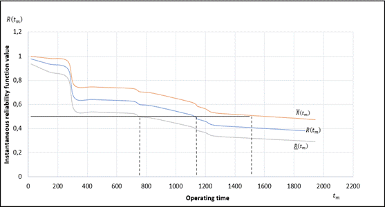
Fig. 1. Reliability function of IAS Components

On the histogram, the estimated quantile of order p=0.5 for the object’s failure-free operating time was marked. From the reliability function plot at p=R=0.5 the corresponding durability values were obtained as T_0,5=1170h, _0,5=1500h, _0,5=780h. This result indicates that, at a confidence level of β=0.95, the object’s reliability in the time interval [780, 1500] will be R(t_m)=0,5.

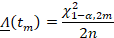
The next step was to estimate the expected value of the leading distribution function and the corresponding confidence intervals [, , β=0,95], based on formulas:

(5)

(6)

(7)

Using the estimated values, a results table and a histogram were generated, the latter of which was subjected to polynomial regression in MATLAB.

Tab. 4

Results of the leading distribution function analysis for IAS components

tm [h]	Number of failures [no.]	Cumulative number of failures – m [no.]	Sample size – n [no.]
20	1	1	45	0,022222222	0,00114	0,066572
143	2	3	45	0,066666667	0,018171	0,139907
270	2	5	45	0,111111111	0,043781	0,203412
314	14	19	45	0,422222222	0,276489	0,59315
449	1	20	45	0,444444444	0,294556	0,619539
712	1	21	45	0,466666667	0,312711	0,645823
756	2	23	45	0,511111111	0,349322	0,698107
849	1	24	45	0,533333333	0,367756	0,72412
1105	6	30	45	0,666666667	0,479866	0,878688
1141	2	32	45	0,711111111	0,517721	0,929725
1146	1	33	45	0,733333333	0,536726	0,955166
1203	2	35	45	0,777777778	0,574881	1,005902
1256	3	38	45	0,844444444	0,632442	1,081677
1474	2	40	45	0,888888889	0,671017	1,131989
1846	3	43	45	0,955555556	0,729148	1,207199
1944	1	44	45	0,977777778	0,748591	1,2322

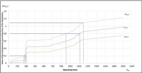
Fig. 2. Leading distribution function of IAS components

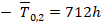
Using the graphical estimation method based on Figure 2, the expected value of the time to the m-th failure and the time interval between the (m-1)-th and m-th failure (corresponding to a 60% resource depletion) were determined, yielding respectively:

, and and

The obtained results provide a numerical representation of the preliminary assessment of object aging by determining the failure-free operating time.

=

(8)

=

(9)

=

(10)

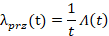
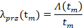
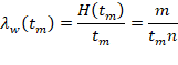
In the subsequent calculations, the Author approximated the aging times of the objects. For this purpose, an estimation of the instantaneous mean failure intensity function of the tested objects, along with the corresponding confidence intervals , , β=0,95 was performed. Using formulas:

(11)

(12)

(13)

The Author prepared Table 5 presenting the research results, as well as Figure (histogram), which was subjected to polynomial regression in MATLAB.

Tab. 5

Results of the instantaneous failure intensity function analysis of IAS components

tm [h]	Number of failures [no.]	Cumulative number of failures – m [no.]	Sample size – n [no.]
20	1	1	45	0,001111111	5,7E-05	0,003329
143	2	3	45	0,0004662	0,000127	0,000978
270	2	5	45	0,000411523	0,000162	0,000753
314	14	19	45	0,001344657	0,000881	0,001889
449	1	20	45	0,000989854	0,000656	0,00138
712	1	21	45	0,000655431	0,000439	0,000907
756	2	23	45	0,000676073	0,000462	0,000923
849	1	24	45	0,00062819	0,000433	0,000853
1105	6	30	45	0,000603318	0,000434	0,000795
1141	2	32	45	0,000623235	0,000454	0,000815
1146	1	33	45	0,000639907	0,000468	0,000833
1203	2	35	45	0,000646532	0,000478	0,000836
1256	3	38	45	0,000672328	0,000504	0,000861
1474	2	40	45	0,000603045	0,000455	0,000768
1846	3	43	45	0,000517636	0,000395	0,000654
1944	1	44	45	0,000502972	0,000385	0,000634

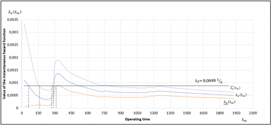
Fig. 3. Instantaneous failure intensity function of IAS components

In the study, a graphical method was applied to estimate the preliminary aging time t_S of the objects with confidence intervals, as well as the preventive maintenance time t_P (after which preventive actions, e.g., component replacement, are carried out), also with confidence intervals.

Assuming the permissible failure intensity value of λ_d = 0,00088 [], the following results were obtained:

The graph shows the presence of extrema. Since the UAV is a complex object, the extrema indicate the existence of weak links within the system. Therefore, it is purposeful to estimate the time of preventive maintenance actions

Looking comprehensively at the selected IAS component through all the obtained research results – namely, the instantaneous reliability function, the instantaneous failure intensity function, and the instantaneous leading distribution function presented in Figure 4 – one can observe their interdependencies.

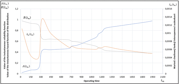
Fig. 4. Comparison of the Instantaneous reliability function, the instantaneous leading distribution function, and the instantaneous failure intensity function for IAS components

At the beginning of the observation (around 100 h), the characteristic curves show a tendency toward stabilization. The Author notes that this is a typical behavior in the early stage of observation, given the short observation time and the limited amount of failure data. Therefore, it was considered justified to conclude that the most failure-prone IAS component begins its aging process already in the initial phase (t_S=55 h).

In the next stage, a distinct extremum is visible, resulting from a significant increase in the instantaneous failure intensity (270-300 h of observation). This, in turn, causes the instantaneous reliability of the objects to decrease sharply by 30%, accompanied by a simultaneous 30% resource depletion. The lower bound of the maintenance window (275 h) corresponds to the lower 95% confidence bound of the preventive maintenance time tP derived from the instantaneous failure intensity function at the permissible threshold λd = 0.00088 [1/h], while the upper bound (314 h) corresponds to the point estimate t_P at which the failure intensity first peaks (see Table 2, cumulative failures reaching 19 out of 45 at tm=314 h). The interval [275, 314] h thus represents the range within which the failure intensity crosses the permissible threshold with 95% statistical confidence. Consequently, it is considered reasonable to carry out preventive maintenance activities within the range of 275-314 h of flight time.

Further observation indicates that at 50% resource depletion (time interval [314-1944 h]), the characteristics tend toward stationarity of the failure process (instantaneous failure intensity, instantaneous reliability, and resource consumption), with one noticeable exception: at 80% resource depletion, a sudden increase in instantaneous failure intensity is observed, along with a 10% drop in reliability. Therefore, defining the object’s failure-free operating time as a reflection of the aging assessment within the 20-80% resource depletion interval was considered justified by the Author, yielding:

= .

(14)

Based on the examination of selected components and the presented graphical solution for estimating the preliminary aging times of Orbiter 2B UAV components, as well as estimating the time frames for carrying out preventive maintenance activities, the Author found it necessary to highlight the potential impact of implementing modern solutions on UAV systems.

The reliability of airspeed indicators in unmanned aircraft is of crucial importance for safe operation, particularly due to the absence of a pilot capable of making real-time decisions. Recent technological advances have led to various methods aimed at enhancing the accuracy and reliability of these indicators. The following sections present the key developments in this field.

5. DISCUSSION

The reliability analysis of IAS sensors in Orbiter 2B UAVs revealed clear aging patterns that align with known vulnerabilities of Pitot-static systems reported in the literature [5, 7, 8]. The results demonstrated a significant increase in failure intensity within the interval of 270-300 flight hours, followed by a stabilization phase, and another failure intensity growth at around 80% resource depletion. This behavior is consistent with the “wear-out” phase of the bathtub curve model, well established in reliability engineering literature for avionic components [11, 13].

The comparison with earlier studies confirms that the main causes of IAS sensor malfunctions – contamination and icing – are dominant in both civil and military applications [1, 3, 5]. The present findings reinforce previous accident investigations (e.g., Air France Flight 447, Birgenair 301) that linked Pitot-tube icing to critical flight incidents [5]. In UAV operations, these risks are amplified by the lack of real-time pilot intervention, which increases the importance of preventive maintenance and sensor redundancy.

A notable contribution of this study is the application of non-parametric methods (Kaplan-Meier and Nelson-Aalen estimators) to UAV reliability data. Unlike parametric models, these methods provided reliable estimates of survival and hazard functions without assuming a predefined failure distribution. The obtained results show good consistency with previous works that applied non-parametric tools to avionics reliability [14, 15], while also demonstrating their suitability for relatively small datasets collected from operational fleets.

From a practical standpoint, the analysis suggests that preventive maintenance actions should be scheduled within the interval of 275-314 flight hours to mitigate the rapid growth in failure intensity. This threshold provides a technical basis for optimizing maintenance intervals, which can improve UAV availability and safety. The findings also highlight the potential of integrating reliability analysis with predictive maintenance frameworks, as proposed in recent studies [2, 16].

Nevertheless, several limitations should be acknowledged. The study was based on a sample of 45 UAVs of a single type (Orbiter 2B), which may limit the generalizability of results to other UAV platforms. Additionally, repair times were excluded from the analysis, which might slightly affect the accuracy of availability estimations. Future research should expand the dataset, include multiple UAV types, and integrate condition monitoring data to refine predictive models.

Overall, the study confirms that IAS sensors represent a critical weak point in UAV avionics. By applying non-parametric reliability methods, this research contributes to the development of evidence-based maintenance policies and supports the implementation of advanced diagnostic and preventive measures in UAV transport and defense operations.

6. CONCLUSIONS

This study investigated the reliability of the Indicated Airspeed (IAS) sensor in Orbiter 2B unmanned aerial vehicles using non-parametric methods. The analysis confirmed that the IAS sensor is one of the most failure-prone components of UAV avionics, with failures constituting the second-largest group of recorded malfunctions in the examined fleet. The results of the reliability function and hazard rate estimation revealed clear aging behavior of the IAS sensor. In particular, a sharp increase in failure intensity was observed between 270 and 300 flight hours, which indicates that preventive maintenance should be introduced within this operational interval.

The dominant failure causes were associated with Pitot-tube contamination and icing, which together accounted for the majority of recorded incidents. These findings are consistent with earlier aviation accident investigations and confirm the environmental vulnerability of the IAS system. By applying non-parametric reliability methods, including the Kaplan-Meier and Nelson-Aalen estimators, the study demonstrated that such approaches are effective in UAV reliability assessment, particularly in situations where datasets are limited and no predefined failure distribution can be assumed.

The results provide a quantitative foundation for the development of predictive maintenance strategies for UAV fleets. Their implementation could contribute to improved operational safety, reduced downtime, and more efficient fleet management. At the same time, it must be emphasized that the study was limited to a single UAV type (Orbiter 2B) and a relatively small dataset. Therefore, future research should expand the scope to include multiple UAV platforms and integrate condition monitoring systems, which would further enhance prediction accuracy.

In conclusion, IAS sensor reliability is a critical determinant of UAV operational safety. The findings highlight the importance of implementing evidence-based maintenance policies and technological improvements, such as anti-icing protection and self-cleaning Pitot systems, to ensure safe and reliable UAV operations in both civil and military transport applications.

References

1. Li Q., Z. Chai, R. Yao, T. Bai, H. Zhao. 2025. „Investigation into UAV Applications for Environmental Ice Detection and Deicing Technology”. Drones 9(1): 5. DOI: https://doi.org/10.3390/drones9010005.

2. Shakhatreh H., A.H. Sawalmeh, A. Al-Fuqaha, Z. Dou, E. Almaita, I. Khalil, N.S. Othman, A. Khreishah, M. Guizani. 2019. „Unmanned Aerial Vehicles: A Survey on Civil Applications and Key Research Challenges”. IEEE Access 7: 48572-48634. DOI: https://doi.org/10.1109/ACCESS.2019.2909530.

3. Cristofaro A., T.A. Johansen, A.P. Aguiar. 2015. „Icing Detection and Identification for Unmanned Aerial Vehicles: Multiple Model Adaptive Estimation”. In: Proceedings of the European Control Conference (ECC): 1445-1451. 2015, Linz, Austria. DOI: https://doi.org/10.1109/ECC.2015.7330736.

4. FAA. 2016. „Chapter 8 – Flight Instruments”. In: Pilot’s Handbook of Aeronautical Knowledge, 8-1–8-40. FAA-H-8083-25B. Washington D.C.: Federal Aviation Administration.

5. Janssen R., R. Hann, T.A. Johansen. 2021. „A review on Pitot tube icing in aeronautics: Research trends”. Flow Measurement and Instrumentation 81: 102033. DOI: https://doi.org/10.1016/j.flowmeasinst.2021.102033.

6. Hann R., C. Bak, T.A. Johansen. 2022. „Aerodynamic degradation of fixed-wing UAVs in glaze and rime icing conditions”. Journal of Aircraft 59(5): 1298-1312. DOI: https://doi.org/10.2514/1.C036751.

7. Sarwar W., A. Panta, M. Klaas, W. Schröder. 2019. „Pitot sensor airflow accuracy and failure risk modeling”. Measurement Science and Technology 30(2): 025007. DOI: https://doi.org/10.1088/1361-6501/aaf3f4.

8. Sundararajan S., D. Enns, I. Kanellakopoulos. 2014. „Diagnosis of Airspeed Measurement Faults for Unmanned Aerial Vehicles”. IEEE Transactions on Aerospace and Electronic Systems 50(3): 1736-1751. DOI: https://doi.org/10.1109/TAES.2014.130338.

9. Stenbakken G., T. Vries, M. Ramírez. 2012. „Diagnosis of UAV Pitot tube defects using statistical change detection”. In: AIAA Guidance, Navigation, and Control Conference: 1-9. 2012, Minneapolis, MN, USA. DOI: https://doi.org/10.2514/6.2012-4750.

10. Cao Y., S.N. Balakrishnan, Y. Fang. 2022. „PCA-based Fault Detection for Aircraft Sensors”. IEEE Transactions on Instrumentation and Measurement 71: 1-12. DOI: https://doi.org/10.1109/TIM.2022.3162468.

11. Tobias P.A., D.C. Trindade. 2011. Applied Reliability. 3rd ed. Boca Raton, FL: CRC Press. ISBN: 978-1-4200-1073-5.

12. Nelson W. 2004. Accelerated Testing: Statistical Models, Test Plans, and Data Analyses. Hoboken, NJ: John Wiley & Sons. ISBN: 978-0-471-69736-7.

13. Dodson B. 2006. The Weibull Analysis Handbook. Milwaukee, WI: ASQ Quality Press. ISBN: 978-0-87389-674-7.

14. Kleinbaum D.G., M. Klein. 2012. Survival Analysis: A Self‑Learning Text. New York: Springer. DOI: https://doi.org/10.1007/978-1-4419-6646-9.

15. Lawless J.F. 2003. Statistical Models and Methods for Lifetime Data. 2nd ed. Hoboken, NJ: Wiley. DOI: https://doi.org/10.1002/9781118033005.

16. Goebel K., B. Saha, A. Saxena. 2017. „A comparison of prognostic algorithms for predicting UAV component reliability”. IEEE Transactions on Reliability 66(3): 887-896. DOI: https://doi.org/10.1109/TR.2017.2674518.

Received 26.12.2025; accepted in revised form 02.06.2026

Scientific Journal of Silesian University of Technology. Series Transport is licensed under a Creative Commons Attribution 4.0 International License

---

[1] The Institute of Logistics and Transport, Polish Air Force University, Dywizjonu 303 nr 35 Street, 08-521 Dęblin, Poland. Email: a.michalska@law.mil.pl. ORCID: https://orcid.org/0000-0002-9292-589X

[2] The Institute of Logistics and Transport, Polish Air Force University, Dywizjonu 303 nr 35 Street, 08-521 Dęblin, Poland. Email: r.brodzik@law.mil.pl. ORCID: https://orcid.org/0000-0001-9303-8785

[3] The Faculty of Transport, Warsaw University of Technology, Koszykowa 75 Street, 00-662 Warszawa, Poland. Email: mariusz.izdebski@pw.edu.pl. ORCID: https://orcid.org/0000-0002-9157-7870