Article
citation information:
Elmaihy, A., Abd El-Latif, M. Performance and sizing
of PEM fuel cells under variable operating conditions for an autonomous
underwater vehicle. Scientific Journal of
Silesian University of Technology. Series Transport. 2026, 131, 63-87. ISSN: 0209-3324. DOI: https://doi.org/10.20858/sjsutst.2026.131.4
Ali ELMAIHY[1], Mohamed ABD El-LATIF[2]
PERFORMANCE AND
SIZING OF PEM FUEL CELLS UNDER VARIABLE OPERATING CONDITIONS FOR AN AUTONOMOUS
UNDERWATER VEHICLE
Summary. Ensuring a reliable
power supply is a key challenge for autonomous underwater vehicles (AUVs),
especially when deeper diving, longer endurance, and extended mission range are
required. Proton exchange membrane (PEM) fuel cells offer a promising solution due
to their high-energy density and quiet operation. This study conducted a
detailed PEM fuel cell model in MATLAB/Simulink to evaluate how operating
conditions affect single-cell electrochemical behavior
and stack-level sizing. The model incorporates activation and ohmic losses to
quantify variations in cell voltage under different temperatures and reactant
supply pressures. Based on these analyses, performance and sizing indices are
derived for a practical AUV power system. Results indicate that increasing
operating temperature from 55°C to 85°C, together with increasing oxygen and
hydrogen supply pressures from 1 to 3 atm, enables a
20% reduction in the required number of cells, directly translating into
similar reductions in stack mass and volume. Moreover, reactant consumption
decreases by 9.5%, improving overall energy efficiency by 9.6%. These findings
demonstrate the strong influence of operating conditions on PEM fuel cell
performance and provide guidelines for optimized sizing of AUV fuel cell power
systems.
Keywords: fuel cell performance, activation over potential, ohmic losses,
operating temperature, supply pressures, AUV
1. INTRODUCTION
Underwater
vehicles, including miniature submarines and autonomous underwater vehicles
(AUVs), are increasingly used in the military and commercial fields. Similar to
AUVs, the power system of AUVs has high requirements for stealth (without
vibration and noise) and long endurance [1]. Because of their low pollution and
energy efficiency, fuel cell vehicles (FCVs) have gained popularity in response
to growing worries about global warming, pollution, and energy consumption [2].
PEMFC
and solid oxide fuel cells (SOFC) can be utilized for AUVs [3,4]. PEMFC is the
recommended option since it performs better and runs at lower temperatures
(below 100°C). Many AUVs currently run on batteries [5], but AUV endurance will
increase with the adoption of fuel cell systems [6,7]. Because the storage
media in fuel cells have a far higher energy density than batteries, they can
outperform them in terms of energy density; nonetheless, the issues arise from
their weights and system sizes [8].
Recent
research indicates that commercial AUVs use batteries to store power.
Battery-powered AUVs with greater endurance and range are significantly bigger
than regular ones, which reduces their utility and increases their space
requirements [5,9]. So, fuel cells are used in the AUV industry. According to
[10], the properties of suitable fuel cell systems are:
- The size of fuel cell systems
must be as small and as light as possible.
- The power output of fuel cell
systems must be in the range of 1 kW to 2 kW.
- Fuel cell systems should be
removable, exchangeable, and replaceable.
The
integration of fuel cell technology into Autonomous Underwater Vehicles for
naval applications presents a compelling avenue for enhanced operational
capabilities, characterized by extended endurance, reduced acoustic signatures,
and improved energy efficiency [11]. However, the realization of these benefits
hinges critically on a comprehensive understanding of the intricate
relationship between fuel cell operating conditions, system size, and overall
performance within the unique constraints imposed by the underwater
environment. AUVs represent a paradigm shift in underwater exploration and data
acquisition, offering unparalleled maneuverability
and the ability to access remote and complex underwater environments without
direct human intervention [12]. The evolution of AUV technology has been driven
by advancements in control systems, communication protocols, and sensory
technologies, enabling increasingly sophisticated missions in challenging
underwater settings [13]. The operational demands of AUVs in naval contexts are
particularly stringent, necessitating robust performance under varying
environmental conditions, including temperature fluctuations, pressure
variations, and exposure to corrosive seawater [14].
The
performance of fuel cells is intricately linked to various operating
conditions, encompassing temperature, pressure, humidity, and reactant
stoichiometry, all of which exert a significant influence on the
electrochemical reaction kinetics, mass transport phenomena, and membrane
properties within the fuel cell stack. Hydrogen energy systems, particularly
those employing PEM fuel cells, have been reviewed for underwater applications,
emphasizing the importance of storage methods and operating parameters in
system design [9]. The literature indicates that hydrogen/oxygen storage
strategies and fuel cell operating conditions are interconnected factors that
determine the overall system size and performance. Proper management of these
parameters can lead to more compact and efficient fuel cell systems suitable
for AUV deployment [9]. Knyazhev and Loshchenkov [15] review various fuel cell types,
emphasizing their performance under different operating conditions. It
highlights how these conditions affect size and efficiency, making them
suitable for naval AUV applications, ensuring extended operational duration and
enhanced cruising range. Mendez et al. [16,17] discussed that fuel cell
operating conditions significantly influence size and performance, emphasizing
the need for compact, efficient systems. It highlights the importance of
optimizing reactant storage and system configurations to enhance endurance and
efficiency in AUV applications. Pielecha [18] analyzed fuel cell performance under various driving
conditions, highlighting that urban, rural, and motorway scenarios
significantly affect power output and losses. It emphasizes the importance of
optimizing operating conditions to enhance fuel cell efficiency and longevity
in applications like AUVs. Tsukioka et al. [19] discussed that fuel cell size
and performance in AUVs are influenced by operating conditions such as
temperature, pressure, and the number of cells in series, which determine
output voltage and efficiency, impacting overall energy generation and
operational capability. Challenges associated with hydrogen fuel cells in
transportation and underwater environments further underscore the necessity of
optimizing operating conditions. These include issues related to durability, efficiency, and system integration, which are directly impacted by temperature,
humidity, and load fluctuations [20]. Addressing these challenges through
advanced energy management strategies, such as high-fidelity simulation models
combined with experimental data, has shown promise in enhancing performance
and reducing system size [21].
Because
PEMFC systems are complex, multimodal, and intricately linked, modeling their properties for design and performance
assessment is difficult. Over the years, significant progress has been made in
comprehending the behavior of PEMFC features using
mathematical modeling [22-34]. Models of integrated
cars with fuel cell stacks are necessary to examine the system behavior under varied load, reagent gas pressure, and
temperature conditions in order to maximize the utilization of PEMFCs [35]. In
the meantime, modeling is becoming more and more
significant in design, analysis, and performance evaluation. Qasem and
Abdulrahman [36] reported that, despite several modeling
approaches used in literature for the prediction of PEMFCs performance,
Amphlett et al.'s mathematical modeling [37,38] was
recognized for its prediction accuracy under different operating conditions.
The majority of models in the literature are supported by experimental work.
Evaluating and comparing the polarization curve derived from both mathematical
and experimental investigations is the most popular validation method. If the
findings of two polarization curves are the same or nearly identical, the model
is reliable [39].
The
objective of this paper is to use MATLAB Simulink to build a fuel cell model
according to [37,38]. Then, select a well-known AUV to ascertain its power
needs. The final result was a block diagram that forms the basis for
forecasting the fuel cell's performance under various operating circumstances.
The second part of the paper investigates the impact of operating conditions on
the sizing of the fuel cell system, as well as the consumption rates of
hydrogen and oxygen, which play a crucial role in determining the overall
endurance of the AUV.
2. FUEL CELL MODEL DESCRIPTION
An electrochemical model that can be
used to predict the behavior of PEMFC is presented in
this section. The optimal simulation results depend on the definition of a set
of parameters used in this mathematical model. The following expression can be
used to define the output voltage of a single cell, Vcell
[22,37,38].
 (1)
(1)
Where  is the Nernst equation, which is an expression
for the electromotive force (EMF) for a given product;
is the Nernst equation, which is an expression
for the electromotive force (EMF) for a given product;  is the
activation overvoltage, which is the amount of voltage used to drive the
reaction;
is the
activation overvoltage, which is the amount of voltage used to drive the
reaction;  is the
ohmic overvoltage, which is the amount of voltage lost to the resistance to
electron flow in the electrodes and the resistance to ion flow in the
electrolyte; the terms of Eq. 1 are discussed in the following sections.
is the
ohmic overvoltage, which is the amount of voltage lost to the resistance to
electron flow in the electrodes and the resistance to ion flow in the
electrolyte; the terms of Eq. 1 are discussed in the following sections.
2.1. Nernst Voltage
The Nernst equation for the reaction
described above:
 (2)
(2)
Where T is the stack temperature in (K),
and  and
and  are the hydrogen and oxygen partial gas
pressures in (atm) at the surface of the catalyst at the anode and cathode,
respectively. At each electrode, two distinct cases need to be taken into
account (for example, the first has an inert diluent in the input flows, either
carbon dioxide in the anode flow or nitrogen in the cathode flow), which will
not be considered here. The flows in the second scenario don't contain any
diluent. So
are the hydrogen and oxygen partial gas
pressures in (atm) at the surface of the catalyst at the anode and cathode,
respectively. At each electrode, two distinct cases need to be taken into
account (for example, the first has an inert diluent in the input flows, either
carbon dioxide in the anode flow or nitrogen in the cathode flow), which will
not be considered here. The flows in the second scenario don't contain any
diluent. So  and
and  will be described as [37].
The first case: diluted H2
and O2:
 (3)
(3)
 (4)
(4)
Where i is the
current density  .
.  and
and  are the total humid gas pressures at both the
anode and the cathode, and are given by:
are the total humid gas pressures at both the
anode and the cathode, and are given by:
 (5)
(5)
 (6)
(6)
Where  and
and  are the total dry gas pressures at both the
anode and the cathode.
are the total dry gas pressures at both the
anode and the cathode.  and
and  are the molar fractions of water in
a gas stream at anode and cathode, respectively, at saturation condition for a
given temperature, and are given by:
are the molar fractions of water in
a gas stream at anode and cathode, respectively, at saturation condition for a
given temperature, and are given by:
 (7)
(7)
 (8)
(8)
The  term is the saturation pressure of
water at the operating temperature T. It is determined in a fuel cell by
the following empirical equation:
term is the saturation pressure of
water at the operating temperature T. It is determined in a fuel cell by
the following empirical equation:
 (9)
(9)
 and
and  are the average molar fractions of nitrogen in
the air stream and carbon dioxide in the hydrogen stream, respectively, and are
given by:
are the average molar fractions of nitrogen in
the air stream and carbon dioxide in the hydrogen stream, respectively, and are
given by:
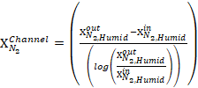 (10)
(10)
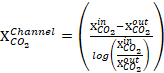 (11)
(11)
 and
and  are the mole fractions of inlet and outlet N2
in the mixture of oxygen and nitrogen, saturated with water vapor, given by:
are the mole fractions of inlet and outlet N2
in the mixture of oxygen and nitrogen, saturated with water vapor, given by:
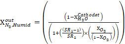 (12)
(12)
 (13)
(13)
 and
and  are the mole fractions of inlet and outlet CO2
in the mixture of Hydrogen and carbon dioxide, and given by:
are the mole fractions of inlet and outlet CO2
in the mixture of Hydrogen and carbon dioxide, and given by:
 (14)
(14)
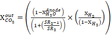 (15)
(15)
SR1 and  are the stoichiometric ratios of oxygen and
hydrogen, respectively.
are the stoichiometric ratios of oxygen and
hydrogen, respectively.  and
and  are the mole fractions of O2 and H2
on the cathode and anode streams, respectively.
are the mole fractions of O2 and H2
on the cathode and anode streams, respectively.
The second case: Pure inlet streams
of H2 and O2:
 (16)
(16)
 (17)
(17)
2.2. Activation overvoltage
Activation losses (also called activation
overpotentials) arise from the energy barrier that must be overcome for the
electrochemical reactions to occur at the electrodes. These losses are more
significant at low current densities. The loss can be decreased if steps are
taken to increase the reaction rates by increasing the temperature or pressure
in the fuel cell, which operates in a temperature range of approximately 55°C
to 85°C. The semi-empirical equation for the activation overvoltage
is given by [37,38]:
 (18)
(18)
Where the
concentration of dissolved oxygen at the gas/liquid interface( ) can be
defined by a Henry’s law expression of the form:
) can be
defined by a Henry’s law expression of the form:
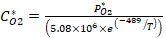
Where the
expression for is given
by Eq. 2.
2.3. Ohmic Overvoltage
Another portion of the voltage generated by
the electrochemical reaction is lost due to the resistance to electron flow in
the electrodes and graphite collector plates, and the resistance to ion flow in
the electrolyte. The ohmic losses can be reduced by using thin, well-hydrated
membranes with high proton conductivity, improving electrical contact, and using materials with low resistivity,
and maintaining proper membrane hydration (dry membranes increase
resistance). The ohmic overvoltage can
be expressed following Ohm’s law as:
 (20)
(20)
Where  is the resistance to electron transfer and is calculated by:
 (21)
(21)
2.4. Fuel Cell Model Implementation
In this paper,
MATLAB/Simulink is used to set up the PEMFC system model. Simulink is a
software package for modeling and simulation, which can be used to evaluate the
system performance and optimize the system design. (Figure 1) shows the
Simulink model of the simulation diagram of the PEMFC dynamic model based on Eqs (1) to (21).
3. MODEL
VALIDATION
To validate the model, a single cell, the Ballard Mark IV model, was
simulated and fed with gases H2 and O2. For oxygen, the
dry-basis mole fraction,  settings were 0.21, 0.46, and 1.00; for hydrogen, , they were 0.65, 0.81, and 1.00. By keeping the total dry gas pressure
at the cathode and anode and
settings were 0.21, 0.46, and 1.00; for hydrogen, , they were 0.65, 0.81, and 1.00. By keeping the total dry gas pressure
at the cathode and anode and  constant at 3.06 atm abs, the partial pressure settings were
accomplished. The stoichiometries of the input flows were maintained at 1.73 cm3
of fuel (anode gas) for every cm3 of hydrogen consumed and 8.33 cm3
of oxidant (cathode gas) per cm3 of oxygen used throughout all runs.
The stoichiometric ratios
constant at 3.06 atm abs, the partial pressure settings were
accomplished. The stoichiometries of the input flows were maintained at 1.73 cm3
of fuel (anode gas) for every cm3 of hydrogen consumed and 8.33 cm3
of oxidant (cathode gas) per cm3 of oxygen used throughout all runs.
The stoichiometric ratios  and are calculated for validation by:
 (22)
(22)
 (23)
(23)
The inlet dry partial
pressure:
 (24)
(24)
 (25)
(25)
The Mark IV employs a Nafion membrane (0.18 mm in
thickness), with an active surface area of 50.56 cm2. Table 1
displays the experimental settings of 28 runs with the corresponding measured
parameters and corresponding predicted results. Comparing diagrams of the total
output voltage, fuel cell resistance, and activation overvoltage between the
model predictions and the experimental data [38] are presented in Figures 2 to
4, respectively. Calculated output voltage response to a range of independent
operating current, temperature, and oxygen partial pressure variations, as
shown in the experimental settings shown in Table 1.
It is demonstrated that the model accurately predicts fuel cell voltage
for current densities as high as 0.33 A/cm2 in the temperature range
of 55 to 85 degrees Celsius and correlates fuel cell voltage over the
experimental range of current densities. In conclusion, the modeling strategy
is found to be successful, efficient, and simple to use with a limited quantity
of data.
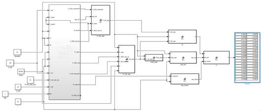
Fig. 1. The block diagram of the MATLAB/SIMULINK model of PEMFCs
Tab. 1
Experimental settings
and comparison between measured values and predicted results
|
Measured Results |
Predicted results |
% Error |
||||||||
|
Run No. |
T [K] |
I [Amp] |
|
|
Vcell [volt] |
Rint [Ω] |
Vcell [volt] |
Rint [Ω] |
Vcell |
Rint |
|
1 |
358 |
2.72 |
0.46 |
0.81 |
0.91 |
0.00388 |
0.916 |
0.00374 |
-0.66 |
3.61 |
|
2 |
328 |
6.66 |
0.21 |
0.81 |
0.773 |
0.00489 |
0.775 |
0.00510 |
-0.26 |
-4.29 |
|
3 |
343 |
6.66 |
0.46 |
0.81 |
0.82 |
0.00455 |
0.823 |
0.00458 |
-0.37 |
-0.66 |
|
4 |
358 |
6.66 |
1 |
0.81 |
0.867 |
0.0041 |
0.869 |
0.00405 |
-0.23 |
1.22 |
|
5 |
343 |
6.66 |
1 |
1 |
0.851 |
0.00453 |
0.856 |
0.00458 |
-0.59 |
-1.10 |
|
6 |
343 |
6.66 |
0.21 |
0.65 |
0.781 |
0.00455 |
0.784 |
0.00458 |
-0.38 |
-0.66 |
|
7 |
328 |
6.66 |
0.46 |
0.65 |
0.802 |
0.00489 |
0.800 |
0.00510 |
0.25 |
-4.29 |
|
8 |
343 |
2.72 |
0.21 |
0.81 |
0.863 |
0.0042 |
0.867 |
0.00426 |
-0.46 |
-1.43 |
|
9 |
343 |
6.66 |
0.46 |
0.81 |
0.824 |
0.00446 |
0.823 |
0.00458 |
0.12 |
-2.69 |
|
10 |
343 |
6.66 |
0.46 |
0.81 |
0.827 |
0.00441 |
0.823 |
0.00458 |
0.48 |
-3.85 |
|
11 |
328 |
2.72 |
0.46 |
0.81 |
0.888 |
0.00495 |
0.882 |
0.00479 |
0.68 |
3.23 |
|
12 |
328 |
6.66 |
1 |
0.81 |
0.835 |
0.00505 |
0.833 |
0.00510 |
0.24 |
-0.99 |
|
13 |
343 |
6.66 |
0.46 |
0.81 |
0.826 |
0.00437 |
0.823 |
0.00458 |
0.36 |
-4.81 |
|
14 |
358 |
6.66 |
0.21 |
0.81 |
0.809 |
0.00406 |
0.805 |
0.00405 |
0.49 |
0.25 |
|
15 |
358 |
6.66 |
0.46 |
1 |
0.846 |
0.00393 |
0.844 |
0.00405 |
0.24 |
-3.05 |
|
16 |
358 |
6.66 |
0.46 |
0.65 |
0.836 |
0.00399 |
0.833 |
0.00405 |
0.36 |
-1.50 |
|
17 |
343 |
16.33 |
0.46 |
1 |
0.715 |
0.00477 |
0.713 |
0.00535 |
0.28 |
-12.16 |
|
18 |
343 |
16.33 |
1 |
0.81 |
0.73 |
0.00493 |
0.736 |
0.00535 |
-0.82 |
-8.52 |
|
19 |
343 |
6.66 |
0.46 |
0.81 |
0.823 |
0.00456 |
0.823 |
0.00458 |
0.00 |
-0.44 |
|
20 |
343 |
6.66 |
0.21 |
0.81 |
0.792 |
0.00441 |
0.790 |
0.00458 |
0.25 |
-3.85 |
|
21 |
358 |
16.33 |
0.46 |
0.81 |
0.729 |
0.00442 |
0.727 |
0.00483 |
0.27 |
-9.28 |
|
22 |
343 |
2.72 |
0.46 |
1 |
0.901 |
0.00428 |
0.904 |
0.00426 |
-0.33 |
0.47 |
|
23 |
343 |
6.66 |
1 |
0.65 |
0.847 |
0.00444 |
0.844 |
0.00458 |
0.35 |
-3.15 |
|
24 |
343 |
2.72 |
0.46 |
0.65 |
0.898 |
0.00428 |
0.893 |
0.00426 |
0.56 |
0.47 |
|
25 |
343 |
16.33 |
0.21 |
0.81 |
0.662 |
0.00477 |
0.676 |
0.00535 |
-2.11 |
-12.16 |
|
26 |
343 |
6.66 |
0.46 |
0.81 |
0.822 |
0.00456 |
0.823 |
0.00458 |
-0.12 |
-0.44 |
|
27 |
328 |
6.66 |
0.46 |
1 |
0.807 |
0.00502 |
0.812 |
0.00510 |
-0.62 |
-1.59 |
|
28 |
343 |
16.33 |
0.46 |
0.65 |
0.7 |
0.0049 |
0.702 |
0.00535 |
-0.29 |
-9.18 |


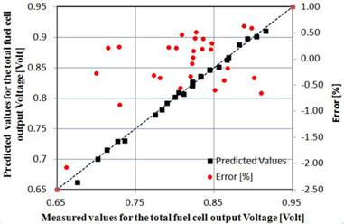
Fig. 2. Parity plot of the model prediction and the measured values for
the total output voltage
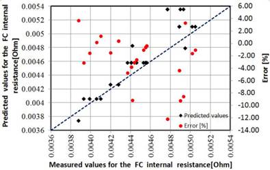
Fig. 3. Parity plot of the model prediction and the measured values for
the FC internal resistance
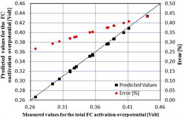
Fig. 4. Parity plot of the
model prediction and the measured values
for the FC activation overpotential
This section aims to present a procedure for obtaining the most suitable
operating conditions for the fuel cell to power an AUV. The inferred
requirements of FCs for AUVs are mentioned in [5]. The proposed procedure is
summarized as follows:
1.
Selection of the AUV.
2.
Estimation of the required
power for the selected AUV.
3.
Prediction of the
performance of one cell of Ballard IV FC (cell output voltage and power) at
different operating conditions, namely, Cell temperature, H2 supply
pressure, and O2 supply pressure at different current densities.
4.
Recording the maximum power
and the corresponding current density for each operating condition ( ,
,  and T).
5.
Calculations of the number
of cells needed to produce the AUV's required power at each operating
condition.
6.
Calculation of the H2
and O2 consumption,
7.
Calculation of the FC
efficiency.
8.
Analysis of the obtained
results.
Figure 5 presents a
flowchart illustrating the previously described procedures.
4.1. AUV
Selection and Required Power Estimation
The AUV ECA A27-E [5,40] is a Classical rear propeller with control
surface architectures, such as in large conventional submarines equipped with
rudders, which take an important place in the AUV market since it has a great
performance following straight lines due to its torpedo-shaped hull. The main
characteristics of A27-E AUV are shown in Table 2.
The viscous resistance coefficient CV, the friction
resistance coefficient CF, and the shape factor (1+ k)
are used to calculate the power consumption of propulsion engines.
CF can be calculated using the
International Towing Tank Conference 57 correlation line (ITTC, 1957) [41]:
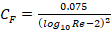 (26)
(26)
Where Re is the Reynolds Number based on the AUV length and speed:
Re= (27)
(27)
Where: μ is the kinematic viscosity of seawater [m2/s];
L is the length of ROV [m]; v is the calculated speed of ROV
[m/s]. For AUVs with a circular cross-section, Droblenkov's
curve can be used to determine the form coefficient:
 (28)
(28)
Thus, viscous resistance is calculated by the expression:
 (29)
(29)
Where: ρ = 1025 [kg/m3]- density of seawater; A is
the wet surface area of the ROV, calculated as a cylinder of diameter D
and length L. The required thrust power is calculated by:
 (30)
(30)
Where ηD is the
propeller thrust performance.
Figure 6 shows the dependence of AUV resistance and required thrust power
on the AUV speed. At the maximum AUV speed, the required thrust power is 1523
W.
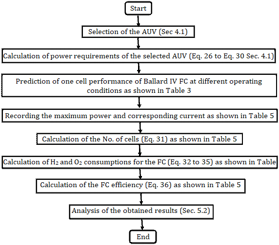
Fig. 5. Flow diagram of the method presented
for sizing the AUV fuel cell
and calculating the gas consumption at different operating conditions
Tab. 2
Main Characteristics of
A27-E AUV [5]
|
Parameters |
Value |
|
Length |
4.5 m |
|
Diameter |
0.73 m |
|
Weight |
850 kg |
|
Maximum diving depth |
300 m |
|
Maximum speed |
6 knotes-3.09 m/s |
|
Underwater endurance at speed 6 knots |
30 hr |
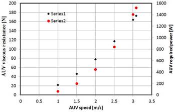
Fig. 6. Viscous resistance power requirement at different AUV speeds
4.2. Single FC at
different operating conditions
The mathematical model described in Section II is used to predict the
performance of one cell of Ballard IV FC at different operating conditions.
Pure oxygen systems are usually exclusively utilized in situations when air is
unavailable, such as submarines and other vessels, due to technical challenges,
the additional bulk and weight of air storage, and associated safety
considerations [42].
The operating
conditions selected in this study are consistent with those commonly reported
for PEM fuel cells used in AUV and underwater applications. Specifically, the
temperature range of 55-85°C aligns with the operating range of PEM fuel cells
[10,11, 27] and the typical operating window of Nafion-based
PEM fuel cells (60-80°C), where high proton conductivity and stable membrane
performance are achieved [25]. Similarly, the selected hydrogen and oxygen
inlet pressures (1-3 atm) fall within the commonly adopted range in the
literature [27], where moderate pressurization improves reactant availability
and reduces mass transport losses without imposing excessive compression
penalties or safety risks, as discussed in [43]. Therefore, these ranges
represent a practical compromise between performance, efficiency, system
compactness, and operational safety, making them suitable for AUV applications
and consistent with established literature.
Table 3 shows 36 combinations of different operating conditions with a
special designation that is developed to enable straightforward identification
and correlation with the operating conditions. The designation is OIHJTM where
O is for oxygen, I is the inlet dry pressure of O2 [atom], H is for
hydrogen, J is inlet dry pressure of H2 [atom], T is for operating
cell temperature and M is the value of the temperature [oC]
so O1H3T60 means a case in which the inlet oxygen dry pressure is 1 atom, the
inlet hydrogen dry pressure is 3 atoms operating at 60oC. The
stoichiometric ratios SR1 and SR2 are fixed
at 1.4 and 1.25 for oxygen and hydrogen, respectively, for all runs as
recommended by [42].
Tab. 3
Different Calculations Operating Conditions
|
Case |
|
|
T[K] |
Case |
|
|
T[K] |
|
O1H1T55 |
1 |
1 |
55 |
O1H1T75 |
1 |
1 |
75 |
|
O1H2T55 |
1 |
2 |
55 |
O1H2T75 |
1 |
2 |
75 |
|
O1H3T55 |
1 |
3 |
55 |
O1H3T75 |
1 |
3 |
75 |
|
O2H1T55 |
2 |
1 |
55 |
O2H1T75 |
2 |
1 |
75 |
|
O2H2T55 |
2 |
2 |
55 |
O2H2T75 |
2 |
2 |
75 |
|
O2H3T55 |
2 |
3 |
55 |
O2H3T75 |
2 |
3 |
75 |
|
O3H1T55 |
3 |
1 |
55 |
O3H1T75 |
3 |
1 |
75 |
|
O3H2T55 |
3 |
2 |
55 |
O3H2T75 |
3 |
2 |
75 |
|
O3H3T55 |
3 |
3 |
55 |
O3H3T75 |
3 |
3 |
75 |
|
O1H1T65 |
1 |
1 |
65 |
O1H1T85 |
1 |
1 |
85 |
|
O1H2T65 |
1 |
2 |
65 |
O1H2T85 |
1 |
2 |
85 |
|
O1H3T65 |
1 |
3 |
65 |
O1H3T85 |
1 |
3 |
85 |
|
O2H1T65 |
2 |
1 |
65 |
O2H1T85 |
2 |
1 |
85 |
|
O2H2T65 |
2 |
2 |
65 |
O2H2T85 |
2 |
2 |
85 |
|
O2H3T65 |
2 |
3 |
65 |
O2H3T85 |
2 |
3 |
85 |
|
O3H1T65 |
3 |
1 |
65 |
O3H1T85 |
3 |
1 |
85 |
|
O3H2T65 |
3 |
2 |
65 |
O3H2T85 |
3 |
2 |
85 |
|
O3H3T65 |
3 |
3 |
65 |
O3H3T85 |
3 |
3 |
85 |
4.3. Fuel Cell Stack for AUV
Using the polarization curve V-I and the power curve  -I for each operating condition, the maximum power for the single FC,
  , is determined with
the corresponding current density and output voltage.
, is determined with
the corresponding current density and output voltage.
The number of cells, NFC, is determined by:
 (31)
(31)
According to the electrochemical reactions of the PEMFC, the molar
consumption of H2 and O2 can be determined as follows.
 (32)
(32)
 (33)
(33)
The inlet mass flow rate of H2 and O2 in gm/s is
calculated by:
 (34)
(34)
 (35)
(35)
Where  and
and  are the molar masses of hydrogen
and oxygen.
are the molar masses of hydrogen
and oxygen.
The fuel cell energy efficiency is calculated by [44]:
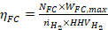 (36)
(36)
5. RESULTS and DISCUSSIONS
5.1. Single FC at Different
Operating Conditions
The impact of operating supply pressure of H2 and O2
on PEMFC performance is assessed and displayed in Figures 7 to 11. Anode and
cathode gas supply conditions are examined under various combinations of and as shown in Table 3. The maximum
power for all cases occurs at a current range of 36.5 A and 41.75 A,
corresponding to a current density of 0.72 A/cm2 and 0.83 A/cm2,
respectively. The output voltage and power at a current of 40 A are displayed
in Table 4 and will be used for comparisons. Table 4 demonstrates the output
cell voltage and power at 40 A and operating temperatures of 55°C
and 85°C.
Tab. 4
The output cell voltage and
power at 40 A and operating temperatures of 55°C and 85°C
|
Case |
|
|
T[K] |
V [V] |
|
Case |
|
|
T[K] |
Vcell[V] |
|
|
O1H1T55 |
1 |
1 |
55 |
0.401 |
16.043 |
O1H1T85 |
1 |
1 |
85 |
0.458 |
18.308 |
|
O1H2T55 |
1 |
2 |
55 |
0.411 |
16.424 |
O1H2T85 |
1 |
2 |
85 |
0.467 |
18.696 |
|
O1H3T55 |
1 |
3 |
55 |
0.416 |
16.650 |
O1H3T85 |
1 |
3 |
85 |
0.473 |
18.933 |
|
O2H1T55 |
2 |
1 |
55 |
0.423 |
16.912 |
O2H1T85 |
2 |
1 |
85 |
0.481 |
19.257 |
|
O2H2T55 |
2 |
2 |
55 |
0.432 |
17.293 |
O2H2T85 |
2 |
2 |
85 |
0.491 |
19.645 |
|
O2H3T55 |
2 |
3 |
55 |
0.438 |
17.519 |
O2H3T85 |
2 |
3 |
85 |
0.497 |
19.881 |
|
O3H1T55 |
3 |
1 |
55 |
0.436 |
17.421 |
O3H1T85 |
3 |
1 |
85 |
0.495 |
19.812 |
|
O3H2T55 |
3 |
2 |
55 |
0.445 |
17.802 |
O3H2T85 |
3 |
2 |
85 |
0.505 |
20.200 |
|
O3H3T55 |
3 |
3 |
55 |
0.451 |
18.027 |
O3H3T85 |
3 |
3 |
85 |
0.511 |
20.436 |


Examining how voltage loss responds could help
explain the improvement in cell performance. The activation overpotential does
not exhibit a pressure term. Activation losses are the voltage losses due to
the finite kinetics of the electrochemical reactions at both electrodes, namely
the Oxygen Reduction Reaction (ORR) at the cathode
and Hydrogen Oxidation Reaction (HOR) at the
anode. They reflect the energy barrier that must be overcome for the reactions
to proceed at a given current density. The change in activation overpotential
is influenced by the O2 concentration, which is a function of as shown in
Eq. 19. At a current of 40 A, the reduction percent in activation overpotential
approximately attains 5.4% and 6.4% when  increases from 1 atm to 3 atm, at 55°C
and 85°C, respectively. Gerling
et al. [45] showed that under
controlled O₂ partial pressure conditions, the exchange
current density for ORR increased significantly, causing lower activation overpotential at the cathode. Butori et al. [25] decoupled
the effects of O₂ partial pressure, humidity, and temperature and found
that raising O₂ partial pressure improved voltage stability across
current densities by maintaining
adequate cathode kinetics even at higher temperatures. On the other hand,
increasing does not
affect the activation overpotential as shown in Figures 7a and 7b at
temperatures 55°C and 85°C, respectively. The negligible
effect of overpotential with the partial pressure of H2 is often
true in well-optimized PEMFCs under moderate to high H2 pressures
and moderate current densities, where mass-transport losses are not dominant.
In other regimes (low H2 pressure, high current density, degraded
diffusion layers, transient operation), the effect can be noticeable [46]. The
HOR is often neglected in full cell studies for the sake of simplicity,
justified by the high rates of the kinetics [45].
increases from 1 atm to 3 atm, at 55°C
and 85°C, respectively. Gerling
et al. [45] showed that under
controlled O₂ partial pressure conditions, the exchange
current density for ORR increased significantly, causing lower activation overpotential at the cathode. Butori et al. [25] decoupled
the effects of O₂ partial pressure, humidity, and temperature and found
that raising O₂ partial pressure improved voltage stability across
current densities by maintaining
adequate cathode kinetics even at higher temperatures. On the other hand,
increasing does not
affect the activation overpotential as shown in Figures 7a and 7b at
temperatures 55°C and 85°C, respectively. The negligible
effect of overpotential with the partial pressure of H2 is often
true in well-optimized PEMFCs under moderate to high H2 pressures
and moderate current densities, where mass-transport losses are not dominant.
In other regimes (low H2 pressure, high current density, degraded
diffusion layers, transient operation), the effect can be noticeable [46]. The
HOR is often neglected in full cell studies for the sake of simplicity,
justified by the high rates of the kinetics [45].
Operating temperature has a significant effect on the activation energy
and activation losses of PEMFC. As operating temperature increases, the
reaction kinetics improve, mainly due to faster charge transfer reactions,
increased proton conductivity in the membrane, and reduced activation energy
barrier for the electrochemical reactions. The effect can be understood using
the Arrhenius equation, which shows that increasing operating temperature
results in higher exchange current density and reduced activation
overpotential. The effect of operating temperature is shown in Figures 8a and
8b. When the operating temperature increases from 55°C to 85°C,
the percentage decrease of activation overpotential is 7.84% at both O2
and H2 supply pressures of 1 atm and 8.82% at both O2 and
H2 supply pressures of 3 atm
|
|
|
|
a) |
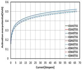
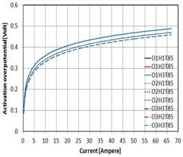
Fig. 7.
Effect of and on the activation overpotential at operating temperatures of 55°C
and 85°C
|
|
|
|
a) |
b) |
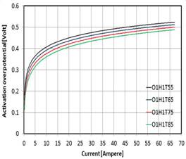
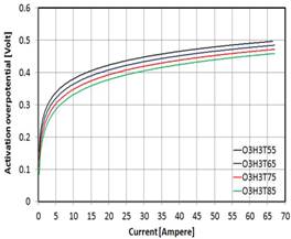
Fig. 8.
Effect of different operating
temperatures on the FC ohmic losses at and of 1 and 3 atoms
The ohmic overpotentials do not exhibit a pressure term. At higher
operating temperatures, water activity and water content of the membrane, and
as a result, membrane conductivity increases and ohmic loss decreases [47,48].
Figure 9 indicates that the ohmic losses decrease as the operating temperature
increases at all O2 and H2 supply pressures. When the
operating temperature increases from 55°C to 85°C, the
percentage decrease of ohmic losses is 13.5% at all O2 and H2
supply pressures.
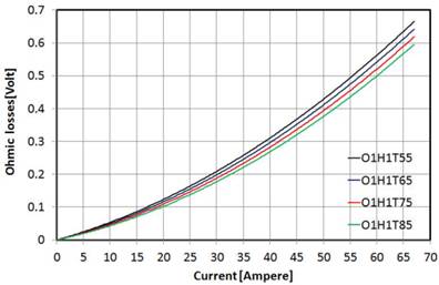
Fig. 9. Effect of different
operating temperatures on the FC ohmic losses at all values of and
The cell output voltage depends on the open circuit voltage and
overpotentials. The open circuit voltage of a fuel cell depends directly on the
reactants' partial pressures, as shown in Eq. 2. When O2
and H2 partial pressures increase, the logarithmic term becomes larger, raising the equilibrium cell
potential. This reduces the relative magnitude of the overpotential (difference between actual voltage and
theoretical voltage). The percentage increase of the Nernst voltage is about
1.3% when increases from 1atm to 3 atm at
all values of  . On the other hand, the percentage increase of Nernst voltage is about
0.65 % when increases from 1atm to 3 atm at
all values of . Increasing either the inlet
pressure of H2 or O2 can result in a high output voltage,
as seen in Figures 10a, 10c,10e, and 10f, and high-power output as shown in
Figures 10b, 10d, 10f, and 10g. The
increase in the output voltage at a temperature of 55°C when Increases from 1 atm to 3 atm
approximately attain 3.78%, 3.58%, and 3.48% for equal 1 atm, 2 atm, and 3 atm,
respectively. These percentages become 3.41%, 3.24%, and 3.15% at an operating
temperature of 85°C. The increase in the output voltage at a
temperature of 55°C when increases from 1 atm to 3 atm
approximately attains 8.58%, 8.39%, and 8.27% for equal to 1 atm, 2 atm, and 3 atm,
respectively. These percentages become 8.21%, 8.04%, and 7.94% at an operating
temperature of 85°C.
. On the other hand, the percentage increase of Nernst voltage is about
0.65 % when increases from 1atm to 3 atm at
all values of . Increasing either the inlet
pressure of H2 or O2 can result in a high output voltage,
as seen in Figures 10a, 10c,10e, and 10f, and high-power output as shown in
Figures 10b, 10d, 10f, and 10g. The
increase in the output voltage at a temperature of 55°C when Increases from 1 atm to 3 atm
approximately attain 3.78%, 3.58%, and 3.48% for equal 1 atm, 2 atm, and 3 atm,
respectively. These percentages become 3.41%, 3.24%, and 3.15% at an operating
temperature of 85°C. The increase in the output voltage at a
temperature of 55°C when increases from 1 atm to 3 atm
approximately attains 8.58%, 8.39%, and 8.27% for equal to 1 atm, 2 atm, and 3 atm,
respectively. These percentages become 8.21%, 8.04%, and 7.94% at an operating
temperature of 85°C.
The effect of increasing is more pronounced than that of
the H2. The percentage increase in cell voltage when increasing both
and from 1 atm to 3 atm is 12.37% and
11.63 at operating temperatures of 55°C and 85oC
respectively. The same percentage increase applies to the ell output power at
all corresponding operating conditions.
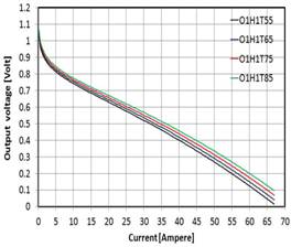
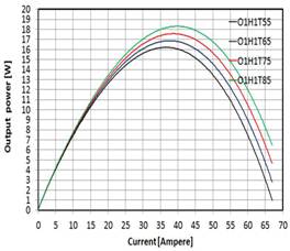
The effect of
operating temperature enhances the fuel cell output voltage and power for all
inlet oxygen and hydrogen supply pressures, as shown in Figures 11a to d. When
the operating temperature increases from 55°C to 85°C,
the increase in the cell output voltage is 14.12% and 13.36% at both and of 1 and 3 atm, respectively.
On the other hand,
open circuit voltage decreases with the increase in operating temperature. As
the operating temperature increases, the Gibbs free energy of the reaction
decreases (1.229 for standard conditions), leading to a lower Nernst voltage.
At the same time, higher temperatures increase the value of RT/2F, which
increases the Nernst voltage. This can partially offset the drop caused
by the decrease in Gibbs free energy, especially in pressurized operation. In
general, the Nernst voltage slightly decreases with temperature under constant
pressure. Results show that when the operating temperature increases from 55°C
to 85°C, the Nernst voltage decreases 2% and 1.85% at
both values of and of 1 atm, 3 atm, respectively. Finally, decreasing ohmic loss and activation overpotential dominate the
Nernst voltage; consequently, the fuel cell performance enhances.
Increases in operating temperature and pressure can improve cell
performance, according to experimental research on the impact of operating
circumstances on cell performance [30]. Therefore, lowering the irreversibility
rate and improving the cell's performance can lower the cost and aid in the
fuel cell's commercialization.
5.2. Fuel Cell Stack for AUV
All calculations
shown by Eqs. 31 to 36 at maximum predicted cell
power under different operating conditions are shown in Table 5. The stack
power for the considered AUV is 1523W.
Tab. 5
Different Calculations at Different Operating Conditions
|
Case |
[W] |
I [Ampere] |
|
O2 Cons. [Mole/s] |
O2 Cons. [gm/s] |
H2 Cons. [Mole/s] |
H2 Cons. [gm/s] |
ηEnergy |
|
O1H1T55 |
16.21 |
36.5 |
94 |
0.0116 |
0.370 |
0.022 |
0.045 |
0.283 |
|
O1H2T55 |
16.56 |
37 |
92 |
0.0115 |
0.367 |
0.022 |
0.045 |
0.286 |
|
O1H3T55 |
16.77 |
37.25 |
91 |
0.0114 |
0.365 |
0.022 |
0.044 |
0.287 |
|
O2H1T55 |
17.01 |
37.25 |
90 |
0.0112 |
0.359 |
0.022 |
0.044 |
0.291 |
|
O2H2T55 |
17.37 |
37.75 |
88 |
0.0111 |
0.357 |
0.021 |
0.043 |
0.294 |
|
O2H3T55 |
17.58 |
38 |
87 |
0.0111 |
0.355 |
0.021 |
0.043 |
0.295 |
|
O3H1T55 |
17.49 |
37.75 |
88 |
0.0111 |
0.354 |
0.021 |
0.043 |
0.296 |
|
O3H2T55 |
17.85 |
38.25 |
86 |
0.0110 |
0.352 |
0.021 |
0.043 |
0.298 |
|
O3H3T55 |
18.07 |
38.25 |
85 |
0.0109 |
0.348 |
0.021 |
0.042 |
0.301 |
|
O1H1T65 |
16.87 |
37.5 |
91 |
0.0114 |
0.365 |
0.022 |
0.044 |
0.287 |
|
O1H2T65 |
17.24 |
38 |
89 |
0.0113 |
0.362 |
0.022 |
0.044 |
0.289 |
|
O1H3T65 |
17.46 |
38.25 |
88 |
0.0112 |
0.360 |
0.022 |
0.044 |
0.291 |
|
O2H1T65 |
17.72 |
38.5 |
86 |
0.0111 |
0.357 |
0.021 |
0.043 |
0.294 |
|
O2H2T65 |
18.10 |
38.75 |
85 |
0.0110 |
0.352 |
0.021 |
0.043 |
0.298 |
|
O2H3T65 |
18.32 |
39 |
84 |
0.0109 |
0.349 |
0.021 |
0.042 |
0.300 |
|
O3H1T65 |
18.23 |
38.75 |
84 |
0.0109 |
0.349 |
0.021 |
0.042 |
0.300 |
|
O3H2T65 |
18.61 |
39.25 |
82 |
0.0108 |
0.346 |
0.021 |
0.042 |
0.302 |
|
O3H3T65 |
18.83 |
39.5 |
81 |
0.0108 |
0.344 |
0.021 |
0.042 |
0.304 |
|
O1H1T75 |
17.57 |
38.75 |
87 |
0.0113 |
0.362 |
0.022 |
0.044 |
0.289 |
|
O1H2T75 |
17.95 |
39 |
85 |
0.0111 |
0.357 |
0.021 |
0.043 |
0.294 |
|
O1H3T75 |
18.18 |
39.25 |
84 |
0.0111 |
0.354 |
0.021 |
0.043 |
0.295 |
|
O2H1T75 |
18.47 |
39.5 |
83 |
0.0110 |
0.351 |
0.021 |
0.043 |
0.298 |
|
O2H2T75 |
18.86 |
40 |
81 |
0.0109 |
0.348 |
0.021 |
0.042 |
0.301 |
|
O2H3T75 |
19.09 |
40 |
80 |
0.0107 |
0.344 |
0.021 |
0.042 |
0.304 |
|
O3H1T75 |
19.01 |
40 |
81 |
0.0108 |
0.345 |
0.021 |
0.042 |
0.303 |
|
O3H2T75 |
19.40 |
40.25 |
79 |
0.0106 |
0.341 |
0.020 |
0.041 |
0.307 |
|
O3H3T75 |
19.63 |
40.5 |
78 |
0.0106 |
0.339 |
0.020 |
0.041 |
0.309 |
|
O1H1T85 |
18.31 |
39.75 |
84 |
0.0111 |
0.356 |
0.021 |
0.043 |
0.294 |
|
O1H2T85 |
18.70 |
40 |
82 |
0.0110 |
0.351 |
0.021 |
0.043 |
0.298 |
|
O1H3T85 |
18.93 |
40.25 |
81 |
0.0109 |
0.349 |
0.021 |
0.042 |
0.300 |
|
O2H1T85 |
19.26 |
40.5 |
80 |
0.0108 |
0.345 |
0.021 |
0.042 |
0.303 |
|
O2H2T85 |
19.66 |
41 |
78 |
0.0107 |
0.342 |
0.021 |
0.042 |
0.306 |
|
O2H3T85 |
19.90 |
41.25 |
77 |
0.0106 |
0.340 |
0.020 |
0.041 |
0.308 |
|
O3H1T85 |
19.83 |
41 |
77 |
0.0106 |
0.339 |
0.020 |
0.041 |
0.309 |
|
O3H2T85 |
20.23 |
41.5 |
76 |
0.0105 |
0.337 |
0.020 |
0.041 |
0.311 |
|
O3H3T85 |
20.48 |
41.75 |
75 |
0.0105 |
0.335 |
0.020 |
0.041 |
0.313 |

The results
indicate a consistent improvement in fuel cell performance with increasing
operating temperature and reactant pressures, which is well aligned with
findings reported by [30,38,49]. As the temperature rises from 55°C to 85°C,
the required number of cells (NFC) decreases significantly
(from 94 to 75), reflecting enhanced reaction kinetics and reduced activation
losses, as discussed in [49]. A similar trend is observed with increasing
O₂ and H₂ pressures, where higher pressurization reduces both oxygen
and hydrogen consumption rates due to improved reactant availability and
reduced mass transport limitations, consistent with observations by [5].
Moreover, the gradual decrease in reactant consumption indicates better fuel
utilization efficiency, which agrees with classical PEMFC performance behavior
reported in [50]. The energy efficiency (ηEnergy)
increases from about 0.283 to 0.313, confirming that elevated temperature and
pressure enhance overall system efficiency, as also highlighted by [42]. Notably, the best performance was
obtained at high temperature (85°C) and high pressures (O3H3).
Overall, the present trends are in strong agreement with established literature
on PEM fuel cell operation.
|
|
|
a) |
b) |
|
|
|
|
c) |
d) |
|
|
|
|
e) |
f) |
|
|
|
|
g) |
h) |
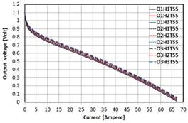
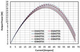
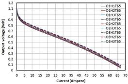
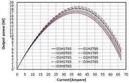
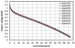
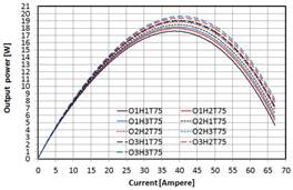
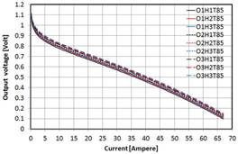
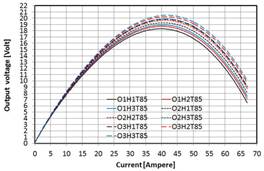
Fig. 10. Effect
of and on the FC output voltage and power
at
different operating temperatures
|
|
|
|||
|
a) |
b) |
|
|
|
|
c) |
d) |
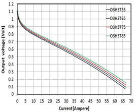
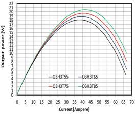
Fig. 11.
Effect of different operating temperatures on the FC output voltage and power at and of 1 and 3 atoms
Results presented in Table 5 show that increasing operating temperature
from 55°C to 85°C and increasing both O2 and H2
supply pressures from 1 to 3 atm result in:
1.
Reduction of the No. of
cells from 94 cells at 1 atm to 75 cells for 3 atm, with a decreasing
percentage of 20%. The percentage is close to the percentage decrease in fuel
cell stack weight and volume.
2.
Reduction of the O2
and H2 consumptions by 9.5%
3.
Increasing the energy
efficiency increases by 9.6%
6.
CONCLUSIONS
The research methodology entails creating a fuel cell model to predict
how different operating conditions affect the performance of a single fuel
cell. The impact of operating conditions on cell voltage losses is investigated
through a comprehensive investigation. Based on these investigations, size and
performance indices are calculated for a fuel cell stack to derive a commercial
AUV under varying operating conditions. The following conclusions can be made
in light of this study:
·
The higher H2 and
O2 supply pressures increase cell performance mainly due to the
decrease in activation overpotential at all current densities and operating
temperatures. On the other hand, they do not affect the ohmic losses.
·
Increasing the cell
operating temperature results in better fuel cell performance, mainly due to
the decrease in both ohmic and activation losses at all current densities and
gas supply pressures.
· The effect of increasing on the FC performance is more
pronounced than that of and .
·
As increases from 1 atm to 3 atm at a
current density of 40 A, the reduction in activation overpotential
approximately attains 5.4% and 6.4%, at 55°C and 85°C,
respectively.
·
The ohmic losses decrease as
the operating temperature increases at both values of and of 1 and 3 atm respectively (ohmic
losses is 13.5% at operating temperature increases from 55°C to 85°C).
·
Concerning the FC stack for
the assigned AUV, the increase of operating temperature from 55°C to
85°C and the increase of both O2 and H2 supply
pressures from 1 to 3 atm result in a reduction of the number of cells by 20%.
This proportion is comparable to the fuel cell stack weight and volume
reduction, with a 9.5% decrease in O2 and H2 consumptions
leading to an increase in the energy efficiency by 9.6%.
References
1.
Wang Z., Z. Liu, L. Fan, Q. Du, K. Jiao. 2023.
,,Application progress of small-scale proton exchange membrane fuel cell’’. Energy
Reviews 2: 10017. ISSN: 2772-9702. DOI: https://doi.org/10.1016/j.enrev.2023.100017.
2.
Chang X., T. Ma, R. Wu. 2019. ,,Impact of urban
development on residents' public transportation travel energy consumption in
China: An analysis of hydrogen fuel cell vehicles alternatives”.
International Journal of Hydrogen Energy 44: 16015-27. ISSN: 1879-3487.
DOI: https://doi.org/10.1016/j.ijhydene.2018.09.099.
3.
Carrette L., K.A. Friedrich, U. Stimming. 2001. ,,Fuel
cells - fundamentals and applications”. Fuel Cells 1(1): 5-39. ISSN: 1615-6854.
DOI: https://doi.org/10.1002/1615-6854(200105)1:1<5::AID-FUCE5>3.0.CO;2-G.
4. Duong, V., N.H. Hiep. 2025. ,,Hybrid propulsion based
on fuel cells”. DTU Journal of Science and Technology 01(68): 3-15. ISSN:
1858-4905.
5.
D'Amore-Domenech R., M.A.
Raso, A. Villalba-Herreros, Ó. Santiago, E. Navarro, T.J. Leo. 2018.
,,Autonomous underwater vehicles powered by fuel cells: Design guidelines”. Ocean
Engineering 153: 387-98. ISSN: 0029-8018. DOI: https://doi.org/10.1016/j.oceaneng.2018.01.117.
6.
Sawa T., T. Aoki,
I. Yamamoto, S. Tsukioka, H. Yoshida, T. Hyakudome,
et al. 2005. ,,Performance of the fuel cell underwater vehicle URASHIMA”. Acoustical
Science and Technology 26(3): 249-56. ISSN: 1346-3962. DOI: https://doi.org/10.1250/ast.26.249.
7.
Hasvold Ø.,
N.J. Størkersen, S. Forseth, T. Lian. 2006. ,,Power sources for
autonomous underwater vehicles”. Journal of Power Sources 162: 935-42. ISSN:
0378-7753. DOI: https://doi.org/10.1016/j.jpowsour.2005.07.021.
8.
Waseem Mohammad,
Mohammad Amir, G.S. Lakshmi, S. Harivardhagini,
Mumtaz Ahmad. 2023. “Fuel Cell-Based Hybrid Electric Vehicles: An Integrated
Review of Current Status, Key Challenges, Recommended Policies, and Future
Prospects”. Green Energy and Intelligent Transportation 2: 100121. ISSN:
2097-2512. DOI: https://doi.org/10.1016/j.geits.2023.100121.
9.
Weydahl H., M. Gilljam, T. Lian, T.C. Johannessen, S.I. Holm, J.Ø.
Hasvold. 2020. ,,Fuel cell systems for long-endurance autonomous underwater
vehicles – challenges and benefits”. International Journal of Hydrogen
Energy 45: 5543-53. ISSN: 1879-3487. DOI: https://doi.org/10.1016/j.ijhydene.2019.05.035.
10.
Farahabadi H.B., M.R. Firuzjaei, A.M. Mir, R. Youneszadeh.
2023. ,,Fuel cell power system conceptual design for unmanned underwater
vehicles”. Hydrogen, Fuel Cell & Energy Storage 10: 33-50. ISSN:
2980-8537. DOI: https://doi.org/10.22104/IJHFC.2022.5884.1248.
11. Cai Q., D.J.L. Brett, D. Browning, N.P. Brandon. 2010.
,,A sizing-design methodology for hybrid fuel cell power systems and its
application to an unmanned underwater vehicle”. Journal of Power Sources
195: 6559-69. ISSN: 0378-7753. DOI:
https://doi.org/10.1016/j.jpowsour.2010.04.078.
12. Sahoo A., S.K. Dwivedy, P.S.
Robi. 2019. ,,Advancements in the field of autonomous underwater vehicle”. Ocean
Engineering 181: 145-60. ISSN: 0029-8018. DOI:
https://doi.org/10.1016/j.oceaneng.2019.04.011.
13. Xiang X., C. Yu, Q. Zhang, P.A. Wilson, G. Xu. 2020.
,,Maneuvering-based actuation evaluation of an AUV
with control surfaces and through-body thrusters”. Applied Ocean Research
96: 102046. ISSN: 0141-1187. DOI: https://doi.org/10.1016/j.apor.2019.102046.
14. Monterroso Muñoz A., M.J. Moron-Fernández, D. Cascado-Caballero, F. Diaz-del-Rio, P. Real. 2023.
,,Autonomous Underwater Vehicles: Identifying Critical Issues and Future
Perspectives in Image Acquisition”. Sensors 23: 4986. ISSN: 1424-8220.
DOI: https://doi.org/10.3390/s23104986.
15. Loshchenkov V.V.K.V. 2024.
,,Fuel Cells for AUV Power Supply”. In: International Conference on Ocean
Studies ICOS. 08-11 October 2024, Vladivostok, Russian Federation. DOI: 10.1109/ICOS63634.2024.10775586.
16. Mendez A., T.J. Leo, M.A. Herreros. 2014. ,,Current
state of technology of fuel cell power systems for autonomous underwater
vehicles”. In: 1st International e-conference Energies. 14-32
March 2014. MDPI: Basel, Switzerland. DOI: https://doi:10.3390/ece-1-d001.
17. Mendez A., T.J. Leo, M.A. Herreros. 2014. ,,Current
state of technology of fuel cell power systems for autonomous underwater
vehicles”. Energies 7: 4676-93. ISSN: 1996-1073. DOI:
https://doi.org/10.3390/en7074676.
18. Pielecha I. 2022. ,,Modeling of fuel cells
characteristics in relation to real driving conditions of FCHEV vehicles”. Energies
15: 6753. ISSN: 1996-1073. DOI: https://doi.org/10.3390/en15186753.
19. Tsukioka S., T. Aoki, I. Yamamoto, H. Yoshida, T. Hyakudome, T. Sawa, et al. 2005. ,,The PEM fuel cell system
for autonomous underwater vehicles”. Marine Technology Society Journal
39(3): 56-64. ISSN: 0025-3324. DOI: https://doi.org/10.4031/002533205787442558.
20. Fakhreddine O., Y. Gharbia, J.F. Derakhshandeh, A.M.
Amer. 2023. ,,Challenges and solutions of hydrogen fuel cells in transportation
systems: a review and prospects”. World Electric Vehicle Journal 14:
156. ISSN: 2032-6653. DOI: https://doi.org/10.3390/wevj14060156.
21. Deutsch C., A. Chiche, S. Bhat, C. Lagergren, G.
Lindbergh, and J. Kuttenkeuler. 2022. ,,Evaluation of
energy management strategies for fuel cell/battery-powered underwater vehicles
against field trial data”. Energy Conversion and Management X 14:
100193. ISSN: 2590-1745. DOI: https://doi.org/10.1016/j.ecmx.2022.100193.
22. Mann R.F., J.C. Amphlett, M.A.I. Hooper, H.M. Jensen,
B.A. Peppley, P.R. Roberge. 2000. ,,Development and
application of a generalized steady-state electrochemical model for a PEM fuel
cell”. Journal of Power Sources 86: 173-80. ISSN: 0378-7753. DOI:
https://doi.org/10.1016/S0378-7753(99)00484-X.
23. Corrêa J.M., S. Member, F.A. Farret,
L.N. Canha, M.G. Simões. 2004. ,,An electrochemical-based fuel-cell
model suitable for electrical engineering automation approach”. IEEE
Transactions on Industrial Electronics 51(5): 1103-12. ISSN: 0278-0046.
DOI: https://doi.org/10.1109/TIE.2004.834972.
24. Abdin Z., C.J. Webb, E.M. Gray. 2016. ,,PEM fuel cell
model and simulation in Matlab-Simulink based on
physical parameters”. Energy 116: 1131-44. ISSN: 0360-5442. DOI:
https://doi.org/10.1016/j.energy.2016.10.033.
25. Butori M., Björn
Eriksson, Nikola Nikolic, Carina Lagergren, Goran Lindbergh, Rakel Wreland Lindstrom. 2023. “The effect of oxygen partial
pressure and humidification in proton exchange membrane fuel cells at
intermediate temperature (80-120°C)”. Journal of Power Sources 563:
232803. ISSN: 0378-7753. DOI: https://doi.org/10.1016/j.jpowsour.2023.232803.
26.
Ali M.A., M.E. Mandour, M.E. Lotfy. 2023. ,,Adaptive Estimation of
Quasi-Empirical Proton Exchange Membrane Fuel Cell Models Based on Coot Bird
Optimizer and Data Accumulation”. Sustainability 15: 9071. ISSN:
2071-1050. DOI: https://doi.org/10.3390/su15119017.
27. Pukrushpan J.T., H. Peng, A.G. Stefanopoulou. 2004. “Control-oriented
modeling and analysis for automotive fuel cell”. Journal
of Dynamic Systems, Measurement, and Control 126: 14-25. ISSN: 0022-0434.
DOI: https://doi.org/10.1115/1.1648308.
28. Correa J.M., F.A. Farret,
M.G. Simoes. 2005. ,,Sensitivity analysis of the modeling
parameters used in simulation of proton exchange membrane fuel cells”. IEEE
Transactions on Energy Conversion 20(1). ISSN: 0885-8969. DOI:
https://doi.org/10.1109/TEC.2004.842382.
29. Jia J., Q. Li, Y. Wang, S. Member, Y.T. Cham, S.
Member, et al. 2009. ,,Modeling and dynamic
characteristic simulation of a proton exchange membrane fuel cell”. IEEE
Transactions on Energy Conversion 24(1): 283-91. ISSN: 0885-8969. DOI:
https://doi.org/10.1109/TEC.2008.2011837.
30. Miansari M., K. Sedighi, M. Amidpour, E. Alizadeh, M. Miansari. 2009. ,,Experimental and thermodynamic approach
on proton exchange membrane fuel cell performance”. Journal of Power Sources
190: 356-61. ISSN: 0378-7753. DOI: https://doi.org/10.1016/j.jpowsour.2009.01.082.
31. Barelli L., G. Bidini, F. Gallorini,
A. Ottaviano. 2010. ,,Analysis of the operating conditions influence on PEM
fuel cell performances by means of a novel semi-empirical model”. International
Journal of Hydrogen Energy 36: 10434-42. ISSN: 1879-3487. DOI:
https://doi.org/10.1016/j.ijhydene.2010.06.032.
32.
Haji Shaker. 2011.
,,Analytical modeling of PEM fuel cell I-V curve”. Renewable
Energy 36: 451-58. ISSN: 0960-1481. DOI:
https://doi.org/10.1016/j.renene.2010.07.007.
33. El-Monem A.A.A., A.M. Azmy, S.A. Mahmoud. 2014.
,,Effect of process parameters on the dynamic behavior
of polymer electrolyte membrane fuel cells for electric vehicle applications”. Ain
Shams Engineering Journal 5: 75-84. ISSN: 2090-4479. DOI:
https://doi.org/10.1016/j.asej.2013.05.001.
34. Alrewq M., A. Albarbar. 2016. ,,Investigation into the characteristics of
proton exchange membrane fuel cell-based power system”. IET Science,
Measurement & Technology 10: 200-206. ISSN: 1751-8822. DOI:
https://doi.org/10.1049/iet-smt.2015.0046.
35. Ceraolo M., C. Miulli, A. Pozio. 2003. ,,Modeling static and dynamic behaviour of proton exchange
membrane fuel cells on the basis of electrochemical description”. Journal of
Power Sources 113: 131-44. ISSN: 0378-7753. DOI: https://doi.org/10.1016/S0378-7753(02)00565-7.
36. Qasem N.A.A., Gubran A.Q.
Abdulrahman. 2024. ,,A recent comprehensive review of Fuel Cells: history,
types, and applications”. International Journal of Energy Research 2024.
ISSN: 0363-907X. DOI: https://doi.org/10.1155/2024/7271748.
37. Amphlett J.C., R.M. Baumert, R.F. Mann, B.A. Peppley, P.R. Roberge, T.J. Harris. 1995. ,,Performance modeling of the Ballard Mark IV solid polymer electrolyte
fuel cell; I. mechanistic model development”. Journal of the Electrochemical
Society 142(1): 1-8. ISSN: 0013-4651. DOI: https://doi.org/10.1149/1.2043866.
38. Amphlett J.C., R.M. Baumert, R.F. Mann, B.A. Peppley, P.R. Roberge, T.J. Harris. 1995. ,,Performance modeling of the Ballard Mark IV solid polymer electrolyte
fuel cell; II. empirical model development”. Journal of the Electrochemical
Society 142: 9-15. ISSN: 0013-4651. DOI: https://doi.org/10.1149/1.2043959.
39. Pathapati P.R., X. Xue, J. Tang. 2005. ,,A new dynamic model for predicting
transient phenomena in a PEM fuel cell system”. Renewable Energy 30:
1-22. ISSN: 0960-1481. DOI: https://doi.org/10.1016/j.renene.2004.05.001.
40. Gasparoto H.F., O. Chocron, M. Benbouzid, P.S. Meirelles. 2021. ,,Advances in
reconfigurable vectorial thrusters for adaptive underwater robots”. Journal
of Marine Science and Engineering 9: 170. ISSN: 2077-1312. DOI:
https://doi.org/10.3390/jmse9020170.
41. Chakrabarti
Subrata K. 2005. “Loads and Responses. In Handbook of Offshore Engineering”, edited by
Chakrabarti Subrata K., 133-196. Elsevier Science. ISBN: 978-0-08-044381-2.
DOI: https://doi.org/10.1016/B978-008044381-2.50007-2.
42. Barbir Frano. 2013. PEM Fuel cells: Theory and
practice. Academic Press is an imprint of Elsevier. ISBN: 978-0-12-387710-9.
43. Hoeflinger J., P. Hofmann. 2020. ,,Air mass flow and
pressure optimisation of a PEM fuel cell range extender system”. International
Journal of Hydrogen Energy 45: 29246-58. ISSN: 1879-3487. DOI:
https://doi.org/10.1016/j.ijhydene.2020.07.176.
44. Chitsaz A., M.A. Haghghi, J. Hosseinpour. 2019. ,,Thermodynamic and exergoeconomic analyses of a proton exchange membrane fuel
cell (PEMFC) system and the feasibility evaluation of integrating with a proton
exchange membrane electrolyzer (PEME)”. Energy Conversion and Management
186: 487-99. ISSN: 0196-8904. DOI:
https://doi.org/10.1016/j.enconman.2019.03.004.
45. Gerling C., Matthias Hanauer, Ulrich Berner, K.
Andreas Friedrich. 2022. ,,PEM Single Cells under Differential Conditions: Full
Factorial Parameterization of the ORR and HOR Kinetics and Loss Analysis”. Journal
of The Electrochemical Society 169: 014503. ISSN: 0013-4651. DOI:
https://doi.org/10.1149/1945-7111/ac44ba.
46.
Stühmeier B.M., M.R.
Pietsch, J. Schwämmlein, H.A. Gasteiger. 2021.
,,Pressure and temperature dependence of the hydrogen oxidation and evolution
reaction kinetics on Pt electrocatalysts via PEMFC-based Hydrogen-Pump
Measurements”. Journal of the Electrochemical Society 168: 064516. ISSN:
0013-4651. DOI: https://doi.org/10.1149/1945-7111/ac099c.
47. Askaripour H. 2019. ,,Effect of operating conditions on the performance of a PEM
fuel cell”. International Journal of Heat and Mass Transfer 144: 118705.
ISSN: 0017-9310. DOI: https://doi.org/10.1016/j.ijheatmasstransfer.2019.118705.
48. Zhang J., H. Zhang, J. Wu, J. Zhang. 2013. “PEM Fuel
Cell Testing and Diagnosis”. Elsevier B.V. ISBN: 978-0-444-53688-4. DOI:
https://doi.org/10.1016/B978-0-444-53688-4.00004-8.
49. EG&G Technical Services Inc. 2004. Fuel Cell
Handbook. 7th ed. U.S. Department of Energy. Under Contract No.
DE-AM26-99FT40575.
50. Dicks A.L., D.A.J. Rand. 2018. Fuel Cell Systems
Explained. 3rd ed. John Wiley & Sons Ltd. ISBN: 9781118706978.
Received 09.01.2026; accepted in revised form 04.05.2026

Scientific Journal of Silesian
University of Technology. Series Transport is licensed under a Creative
Commons Attribution 4.0 International License