Article
citation information:
Ślesicka, A., Ślesicki,
B. The use of deep learning for military vehicle identification in SAR imagery.
Scientific Journal of Silesian University
of Technology. Series Transport. 2025, 128,
251-268. ISSN: 0209-3324. DOI: https://doi.org/10.20858/sjsutst.2025.128.14
Anna ŚLESICKA[1],
Błażej ŚLESICKI[2]
THE USE OF DEEP
LEARNING FOR MILITARY VEHICLE IDENTIFICATION IN SAR IMAGERY
Summary. Artificial intelligence
approaches, especially those involving deep learning, have recently become
integral to object detection, as they can autonomously identify relevant
features in visual datasets. The identification of military equipment,
including mechanized vehicles, is crucial for threat detection and minimizing
the impact of enemy actions by enabling countermeasures to be taken as quickly
as possible after the threat is detected. The application of deep learning,
particularly convolutional neural networks (CNN), is a highly effective tool
for image processing and pattern recognition in visual data. These networks
utilize convolutional layers to automatically extract features from images,
making them ideal for analyzing synthetic aperture
radar (SAR) imagery. Active sensor technologies like SAR are essential for
object recognition due to their capability to operate in all weather
conditions, both day and night.
Keywords: artificial intelligence, convolutional neural networks, SAR radar,
military equipment
1. INTRODUCTION
The
growing adoption of artificial intelligence in numerous fields is closely
linked to the rapid development of deep learning methods. These algorithms,
which rely on deep neural network architectures, are capable of autonomously
extracting features and classifying data. As a result, they have become
essential tools in image analysis, including tasks such as object detection,
image classification, and semantic segmentation [1]. Synthetic Aperture Radar
(SAR) is an important active sensor for microwave imaging, whose ability to
operate around the clock and in all weather conditions makes it a crucial tool
in the remote sensing community [2]. Since the launch of the first SAR
satellite by the United States, this technology has gained widespread
recognition and application in fields such as geological exploration,
topographic mapping, disaster forecasting, and traffic monitoring. Deep
learning-based approaches to SAR data analysis contribute to notable
advancements in the automation of object detection and classification.
Convolutional neural networks can learn both low- and high-level features from
raw images, making them ideal for remote sensing tasks. The use of this
technology in object detection on SAR imagery opens up new perspectives in
terms of the accuracy and efficiency of recognition processes [3].
In
the publication by Majumder, Blasch, and Garren [4], the focus is on analyzing modern deep learning approaches for Automatic
Target Recognition (ATR) on SAR images. The book explores how various neural
networks perform when tested on the MSTAR (Moving and Stationary Target
Acquisition and Recognition) dataset, which was originally developed by DARPA (Defense Advanced Research Projects Agency) and the Air
Force Research Laboratory to support target recognition research. This dataset
contains 20,000 SAR image fragments depicting 10 types of military objects,
including those from the former Soviet Union [5]. Although the MSTAR dataset is
commonly used to evaluate traditional machine learning algorithms, such as SVM,
achieving high classification accuracy (97% - 100%), there are studies
indicating decreased performance of algorithms when tested on other datasets,
such as QinetiQ [6].
In
addition, this work surveys current ATR techniques, with particular emphasis on
neural networks utilizing SAR datasets like MSTAR and TerraSAR-X
as input.
Among
the proposed approaches is the all-convolutional network (A-ConvNet)
proposed by Chen et al., which features high computational efficiency through
the use of sparsely connected convolutions and the omission of the fully
connected (FC) layer [7]. Additionally, Furukawa et al. proposed the VersNet network, which allows for processing SAR images of
various sizes and composed of multiple objects of different classes [8]. Shang
et al., introduced the M-Net model, which utilizes a memory module to predict labels
of unknown samples based on the spatial similarity information of features [9].
In
the domain of SAR image sequence processing, Zhang et al. proposed the MA-BLSTM
framework, which leverages Gabor filters and TPLBP operators for extracting
both global and local information, while utilizing Long Short-Term Memory
(LSTM) networks for the purpose of reducing the dimensionality of extracted
features [10]. Bai et al. on the other hand, proposed an LSTM network that
achieved high performance in the presence of noise, indicating its potential in
complex operational environments [11].
Nevertheless,
when SAR meets deep learning, it is necessary to carefully consider how to
utilize this advanced technology optimally. Deep learning abandons traditional,
hand-crafted features in favor of abstract features
extracted by neural networks [12]. It is essential to understand whether the
abstract features extracted by neural networks can fully represent real SAR
data, and whether traditional features, based on mature theories and techniques,
should be completely abandoned.
The article presents a novel concept of applying deep
learning for object identification in SAR radar imagery, analyzing both the
benefits and challenges of integrating these technologies. The focus is on the
selection of network architecture and its properties, known as hyperparameters.
Potential development directions and research in this rapidly evolving field
are also discussed, considering the unique properties of SAR data and the need
for their efficient utilization in combination with deep learning. In summary,
research on deep learning in the context of ATR in SAR imagery is progressing
dynamically, though it faces challenges related to adaptation to different
environmental conditions and practical operational applications.
2. NEURAL
NETWORK ARCHITECTURE
Deep
neural networks are complex, hierarchical structures composed of multiple
nonlinear layers with local connections between them [13]. These layers act as
automatic, unsupervised feature extractors. The extracted features are then
passed to the final part of the network, which typically consists of one or two
layers of a classical neural network with fully connected connections between
layers.
Deep
neural networks are distinguished by their unified structure, serving both as
feature extractor/selector and as the final classifier or regression system.
This relieves the user from the need to define and select the most important
diagnostic features of the analyzed process. Deep
neural networks excel in image and pattern recognition tasks due to their
ability to learn hierarchical features at different levels of abstraction.
These abstraction levels indicate the progression from low-level, fine-grained
features to high-level, more generalized representations extracted from the
input data. As the signal passes through successive layers of the neural
network, the feature extractors in these
layers learn increasingly complex and abstract representations of the data
[14].
2.1. Database
In
this research, model training and evaluation were conducted using the MSTAR
dataset, which includes 20,000 SAR image patches of various military vehicles
and targets. Among them are the D7 bulldozer, BTR60 and BRDM2 armored personnel
carriers, ZSU23-4 anti-aircraft gun, 2S1 self-propelled howitzer, T62 tank,
ZIL131 truck, and the standard calibration target SLICY. In total, the
developed network will be capable of recognizing 8 different types of objects.
The images were acquired at two different depression angles: 15° and 17°, with
various orientations ranging from 190 to 300, providing comprehensive coverage
of orientations across the entire 360° angle. Figure 1 shows sample SAR radar
data, while Figure 2 illustrates sample objects as seen by optical sensors
like cameras and in SAR imagery.
Among
the most frequently utilized datasets for developing deep learning models in
SAR target identification is the MSTAR database. It is valued for its richness
and diversity of data, enabling researchers to train and test algorithms under
realistic conditions. This database is crucial for developing techniques such
as data augmentation, transfer learning, and assessing the impact of noise and
interference on ATR algorithm effectiveness. In many studies using the MSTAR
dataset, various neural network architectures have been compared, ranging from
smaller networks like LeNet to more advanced ones such as ResNet18 and wide
networks like Wide-ResNet18 [15]. One of the main findings was that more
complex and deeper network architectures do not always translate into higher
effectiveness in SAR target recognition [16].

Fig. 1. Examples of SAR radar images of various objects from
the MSTAR database
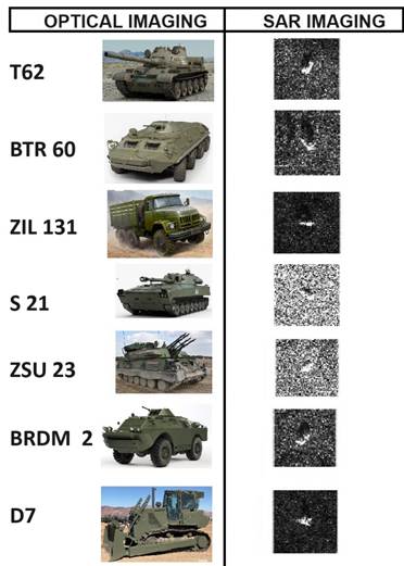
Fig. 2.
Objects imaged using optical and SAR sensors.
2.2 CNN
Network Structure
The
article applied a CNN model, which has a deep, multi-layer structure. The name
CNN stands for Convolutional Neural Network, derived from the convolution
operation, which is a key computational process in these networks. The
convolution of discrete signals can be represented mathematically as described
by the formula in reference [17]:
![]() (1)
(1)
In
the presented equation, x(n) denotes
the input signal, w(n) corresponds
to the convolution kernel, and the resulting output y(n)
forms the feature map. For one-dimensional neural signal processing, the data
are represented as vectors, where x stands for the set of
training signals, and w is a multi-dimensional weight matrix that
adjusts during the learning process. When dealing with images, data are
represented as a two-dimensional matrix I, with each element I(m,
n) indicating the pixel intensity.
The
kernel K also takes the form of a two-dimensional matrix. The
convolution operation for two-dimensional matrices is defined by the formula
[18]:
![]() (2)
(2)
![]() (3)
(3)
Two-dimensional
convolution involves sliding the kernel K over the image matrix I
and computing the sum of element-wise products. The result of this operation is
a new matrix that contains information about how well the kernel K
fits different parts of the image I. Therefore, in Figures 3 and
4, the convolution operation for the image and the filter is depicted.
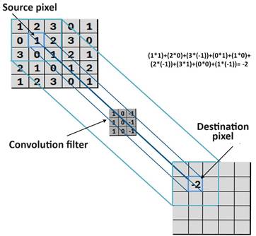
Fig. 3. Example of convolution of a 5x5 image matrix with a
3x3 filter - matrix example
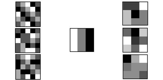
Fig. 4. Example of convolution of a 5x5 grayscale image matrix
with a 3x3 filter
This
is a fundamental operation in convolutional neural networks (CNNs), used to
detect various features in images such as edges, textures, and other patterns.
The convolution operation applied in CNNs offers significant advantages
compared to standard matrix operations in classical neural networks. These
advantages include local connectivity, shared (reusable) filter weights, and
translation invariance (equivariance).
In
neural networks, local connectivity leads to significant savings in the number
of computational operations. Unlike full connectivity, where each neuron is
connected to all input signals, local connections link neurons only to a small
set of neighboring input signals (pixels) within the
range of the convolutional kernel. This kernel typically has much smaller
dimensions than the entire image. Such an approach not only reduces the number
of required computational operations but also lowers the demand for system
memory. Figure 4 illustrates the comparison between full and local weight
connections of neurons with input signals.
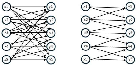
Fig. 5. Example of full (left-side diagram) and local
connection of network neurons
(right-side diagram) in the case of one-dimensional data
Parameter
sharing refers to a technique where the same weights are applied across
different locations in the input. Instead of creating unique sets of weights
for each possible location of the filter mask, the same weights are reused for
different shifts. This practice brings several key benefits. Firstly, it
significantly reduces memory requirements since there is no need to store
separate parameters for each location. This is particularly critical for large
networks or limited hardware resources, where every bit of memory counts.
Secondly, by sharing parameters, the network can more effectively leverage its
learning capacity. Shared weights learn to represent similar features across
different parts of the image or sequence, which can lead to better generalization
and more efficient utilization of knowledge within the network. Additionally,
parameter sharing reduces computational overhead because fewer parameters need
updating during the learning process. This, in turn, speeds up the network
training process and increases its operational efficiency. Overall, parameter
sharing is a significant optimization strategy in neural network design aimed
at improving performance and efficiently utilizing available computational and
memory resources.
Translation
equivariance implies that applying a transformation to the input causes the
output to transform in the same way. In mathematical terms, if function f(x)
is equivariant to function g(x), then f(g(x)) = g(f(x)).
For example, convolving an image shifted one pixel right, I’(x, y) = I(x-1,
y), yields the same result as convolving the original image I(x, y)
and subsequently shifting the output by one pixel.
The
model used in the article includes inter-area convolutional connections in the
initial layers, enabling efficient feature extraction from the input data. The
convolutional layer consists of three levels. The first level involves linear
convolution, which is linear filtering using a moving kernel mask over the
image. The output result is the sum of the linear filtering results of the
previous layer's images, considering different weight values of individual
masks. The next level is the linear activation function, such as ReLU, which operates on the summed output signal of the
linear convolution. The last level involves statistical pooling, which reduces
the image dimensionality by analyzing the results
obtained from the moving filter mask of the neuron. Batch normalization was
applied during training to accelerate learning and stabilize the network [19].
The model also included a pooling layer that helped reduce the dimensionality
of data and improve translation invariance [20]. These features together make
up the CNN architecture shown in Figure 6, which enables effective input
classification.
The
convolutional neural network was designed and implemented in the MATLAB
environment. To conduct the research, a Dell laptop equipped with a 13th
Generation Intel® Core™ i5-1345U processor running at 1.60 GHz, 16 GB of RAM,
and Windows 11 Pro was used. The software tools included MATLAB Version
23.2.0.2365128 (R2023b), developed by MathWorks, Inc., Natick, MA, USA. This
hardware and software configuration provided a reliable platform for the
development, training, and evaluation of the CNN model.
After
extensive preliminary experimentation, the final design of the network settled
on a deep architecture composed of six convolutional layers. It begins
with two layers, each containing 32 neurons and equipped with 3×3 filters that
scan the input with a fine 1×1 stride. These layers are enhanced with batch
normalization and the ReLU activation function,
followed by 2×2 max pooling to efficiently reduce spatial dimensions while
preserving crucial features. As the network progresses deeper, the third and fourth
layers increase the complexity by doubling the neuron count to 64, while
maintaining the proven filter size and stride. This pattern continues in the
fifth and sixth layers, where 128 neurons work in tandem with the consistent
filter and stride settings, batch normalization, and ReLU
activations, capped off with max pooling to compact the learned
representations. This carefully crafted progression enables the network to
extract increasingly abstract and high-level features, laying a strong
foundation for accurate and robust classification.
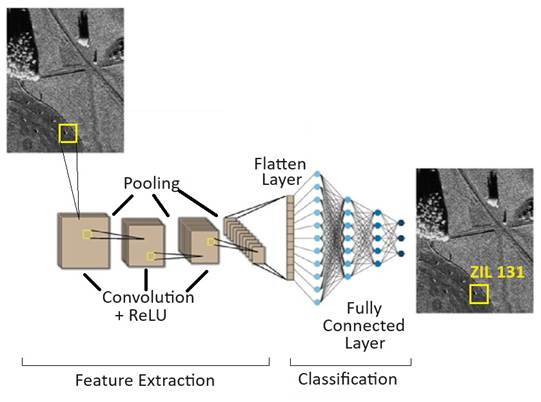
Fig. 6. The architecture of the proposed CNN
The
flatten layer then converts the input feature maps into a one-dimensional
vector, allowing the data to be processed by the fully connected layers. This
fully connected layer contains 8 neurons, representing the eight image
categories, with the Softmax activation function
applied at the output layer for classification purposes.
The
input layer in a convolutional neural network serves as the initial stage that
receives the raw input data. It does not apply any convolutional or activation
functions. Its primary function is to accept the incoming data and forward it
unchanged to the next layers in the network, preserving the original shape and
characteristics of the input. Essentially, it acts as the entry point for data
processing within the neural network [21].
Batch
normalization is a technique designed to mitigate the internal covariate shift
phenomenon, where the distribution of inputs to neural network layers shifts
during training, complicating the learning process. It operates by normalizing
the inputs within each mini-batch: for every feature, it calculates the mean
and standard deviation, then scales the data to have zero mean and unit
variance [22]. This normalization ensures that despite ongoing updates to the
model’s parameters, the input to each layer remains stable, which accelerates
convergence and enhances overall training performance.
After
each convolutional layer in the model, a ReLU
activation function is applied:
![]() (4)
(4)
This
is currently the most widely used activation function for training neural
networks designed for image object recognition. A comparison of various
activation functions commonly used in neural networks is presented in Figure 7.
The
ReLU activation function mitigates the vanishing
gradient problem and makes the network more robust against improper
initialization of parameters. Its operation involves eliminating negative
values, which accelerates network training and enhances its ability to capture
complex data dependencies. This stems from its infinite response to positive
signals and zeroing out negative signals. This approach results in only a
subset of neurons being active during training, which helps prevent overfitting
and accelerates the learning process. Moreover, the ReLU
activation function allows for simple computation of derivatives, and its
piecewise linear nature facilitates efficient backpropagation for updating
network weights.
After
normalization, the data is processed by a statistical filter called max
pooling, which selects the maximum value within each filter window and reduces
computational load in the following layers. By applying this operation to
non-overlapping subregions, only the most prominent features are retained,
significantly decreasing the volume of data passed on for further processing
without sacrificing the algorithm’s performance. The straightforward mechanism
of this 2×2 max pooling filter is illustrated in Figure 8.
Before
reaching the network's output, the information passes through the Softmax function. This function transforms the input vector
into a normalized vector where values range from 0 to 1. Consequently, the
output layer produces values that can be understood as probabilities. This
allows determining the network's accuracy percentage during its analysis.
Figure 9 illustrates an example of how this function operates.
3. NETWORK
LEARNING PROCESS
The
chapter presents the results of the study on the proposed convolutional neural
network model regarding the tuning of network hyperparameters, particularly
focusing on the learning rate of the network. A confusion matrix of the
obtained results for military object detection
is presented. The accuracy of the proposed method is also compared
comprehensively
with other available methods serving as classifiers for objects in the MSTAR
database using CNN.
3.1 Learning Rate
Activation
function, weight vector, as well as the number and type of neural network
layers, learning rate, and a series of other model settings constitute what is
referred to as hyperparameters, directly influencing the operation of neurons.
Hyperparameter values are selected before each network training. The series of
network trainings is referred to as the network learning process. Therefore,
the learning process involves tuning the hyperparameters of the network model
to achieve optimal performance in carrying out the intended task.
The learning
process of the designed neural network involves presenting successive training
examples to the network input, generating responses, and updating
hyperparameters so that with each iteration, the differences between the
model's response and the expected response are minimized. Consequently, the
goal is to achieve the intended effectiveness while making the network capable
of generating correct responses for examples that were not used during
training.
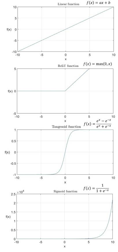
Fig. 7. Overview and Comparison of Activation Functions in
Neural Architectures [23]
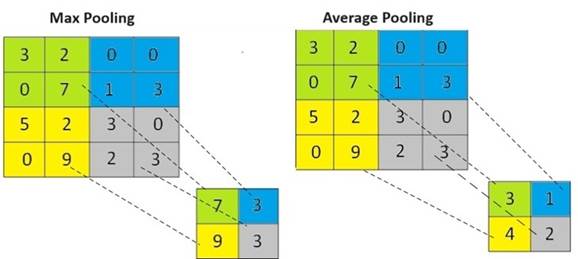
Fig. 8. Comparison of Max Pooling and Average Pooling
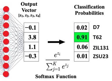
Fig. 9. Operation of the Softmax
function
The learning
rate must be carefully tuned because it has a critical impact on the training
of machine learning models [17]. This parameter determines how large the
maximum weight change of a neuron can be during an update. If this rate is too
small, the learning process becomes very lengthy because the network requires
many iterations to make significant corrections to neuron weights. Conversely,
if the rate is too high, it can lead to excessively large weight corrections,
preventing the network from properly fitting the training data (Figure 10).
When weight
corrections are too large, neuron computations may still exhibit random
behavior even after many iterations of learning, making it difficult for the
network to effectively adapt to input data patterns. When weights are adjusted
in large steps, neuron computations may still exhibit random behavior even
after numerous iterations. In such a situation, it is challenging to fit them
into the overall network pattern, similar to the situation at the beginning of
the learning process.

Fig. 10. Learning process with improperly chosen learning rate
On the other
hand, a properly chosen learning rate (Figure 11) allows the network to quickly
achieve the required accuracy within a few epochs. An epoch denotes a single
pass through all the training examples in the training dataset during the
learning process. Beyond this point, further improvements in recognition
accuracy are minimal.
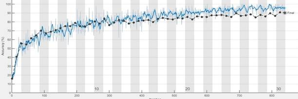
Fig. 11. Training process with an appropriately chosen learning
rate
Setting
the learning rate too high (as shown in Fig. 12) can cause the training process
to advance very quickly, but this rapid progress is not necessarily beneficial.
When the learning rate is excessively large, the network may overshoot the
optimal solution and become stuck in a local minimum, preventing it from
achieving the highest possible recognition accuracy. This underscores the
importance of carefully tuning the learning rate to balance speed and stability
during training.
3.2 Confusion Matrix
Effective
implementation of machine learning requires proper model evaluation, which can
be done quantitatively or qualitatively. Qualitative evaluation of the model
involves analyzing its behavior
and generated outputs. Quantitative evaluation, on the other hand, is based on
metrics that provide information about the correctness of the model's
operation. One of the most popular metrics is accuracy. Accuracy measures how
well the model correctly classifies examples in both binary and multi-class
classification tasks. It ranges from zero (all examples classified incorrectly)
to one (all examples classified correctly). Insights derived from model
evaluation can be used to assess the model's utility and applicability, improve
the training process, identify challenging cases, and select the network
structure and its hyperparameters.
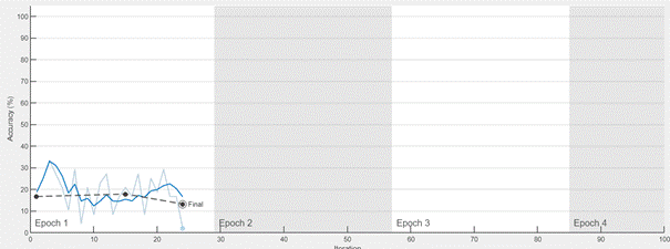
Fig. 12. Training process terminated with an error
In
predictive classifier studies, a particularly useful tool is the confusion
matrix, which provides information about the number and types of errors made,
distinguishing between type I and type II errors:
·
type I
error (false positive, FP) involves rejecting the true null hypothesis, meaning
the presence of an object despite its actual absence;
·
type II
error (false negative, FN) occurs when the false null hypothesis is accepted,
indicating that an object is considered absent even though it is actually
present.
The
confusion matrix stores information about predictions in a table format, where
rows i and columns j represent the true
label and classifier's response, respectively. The value in each cell (i, j) indicates the count of observed
class-prediction pairs. An example matrix for a binary problem is depicted in
Figure 13. The matrix cells contain symbolic notations for TP (true positive),
reflecting correctly classified samples, TN (true negative), indicating
correctly rejected samples, and the errors of types I and II. For the discussed
multiclass classification in the article, the matrix construction needs to be
adjusted to an 8 x 8 size. In this case, redefining TP, FP, FN, and TN
coefficients is required, computed separately for each class i = 1….8. The negative class is considered as
the sum of all classes not analyzed, j = 1…8,
where j ≠ i.
Building
on the neural network architecture outlined above, simulations were carried out
to train a deep neural network capable of classifying eight distinct object
categories. The study employed a dataset of 4,000 images, evenly distributed
with 500 images per class. These images were randomly partitioned into three
subsets: 70% allocated for training to optimize the network’s weights, 15%
reserved for validation to fine-tune the model and prevent overfitting, and the
final 15% set aside for testing to objectively evaluate the network’s
classification performance after training.
Figure 14
presents a confusion matrix that illustrates the performance of the proposed
model across the target classes within the dataset. The matrix highlights
correctly classified instances in blue, while misclassifications are shown in
orange. Notably, the model exhibited difficulties distinguishing the 2S1
vehicle from the T62, ZIL 131, and ZSU 23 vehicles. The simulation results
displayed represent the best outcomes achieved among numerous trials, which
involved extensive and time-consuming experimentation with various parameters,
including the number of images per class, training epochs, and different
hyperparameter settings. A comprehensive summary of all conducted simulations
is provided in Table 3.
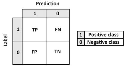
Fig. 13. Definition of the confusion matrix
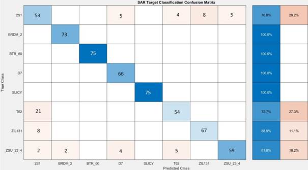
Fig. 14. Simulation results in the form of a confusion matrix
Tab. 1
Summary of all
conducted simulations
|
Simulation 1 |
|
|
Number of images per class |
Accuracy |
|
100 |
71.08 % |
|
200 |
88.54 % |
|
500 |
94.22 % |
|
Simulation 2 |
|
|
Initial learning rate |
Training time |
|
0.00001 |
2060 min |
|
0.0001 |
940 min |
|
0.001 |
250 min |
|
Simulation 3 |
|
|
Initial learning rate |
Accuracy |
|
0.00001 |
66.08 % |
|
0.0001 |
85.54 % |
|
0.001 |
98.22 % |
Figure 15
presents a comparison of the accuracy between the proposed method and the
convolutional neural network structure against other available methods for
recognizing military objects from the MSTAR database depicted using SAR radar
for the same dataset (8 classes with 500 images each). As observed, the method
developed in this article exhibits the highest accuracy.
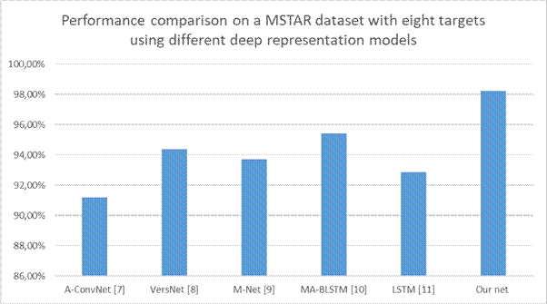
Fig. 15. Comparison of ATR methods accuracies
4. DISCUSSION
AND CONCLUSIONS
This
article proposes an innovative framework for employing deep learning techniques
to identify objects within SAR radar imagery, thoroughly examining the
associated benefits and challenges. Particular attention is given to the
careful selection of the network architecture and its critical hyperparameters,
which play a pivotal role in model performance.
Deep
neural networks and their underlying deep learning techniques have opened new
horizons for advancing artificial intelligence. The innovative fusion of these
technologies with radar systems enables practical applications in everyday
life. By integrating both feature extraction and classification into a single
framework, deep neural networks can process raw data directly, eliminating the
need for manual expert intervention.
The
article explores potential avenues for development and research in this field,
emphasizing the unique advantages of SAR radar – its capability to operate
effectively in all weather conditions and during both day and night. These
features provide engineers with significant opportunities to create advanced
devices for military and civilian uses, including covert monitoring of designated
areas.
The
convolutional neural network model developed in this study was implemented
using MATLAB and rigorously evaluated on the MSTAR dataset, which encompasses
eight different target categories. The experimental results indicate that the
proposed method surpasses most state-of-the-art deep learning models in
accurately recognizing objects within SAR imagery, highlighting its
effectiveness and robustness.
The
authors plan to direct future research towards the practical implementation of
their work, which includes acquiring the necessary SAR radar hardware and UAV
platforms, conducting comprehensive field experiments, and systematically
validating and enhancing the proposed convolutional neural network
architecture.
In
conclusion, the field of deep learning for automatic target recognition (ATR)
in SAR imagery is progressing swiftly, although it still faces significant
challenges in adapting to varying environmental conditions and ensuring
effective performance in practical operational scenarios.
References
1.
Zhao Zhong-Qiu, Zheng Peng, Xu Shou-Tao, Wu Xindong. 2019. „Object detection with deep learning: A
review”. IEEE Transactions on Neural
Networks and Learning Systems, 30(11): 3212-3232. DOI:
10.1109/TNNLS.2018.2876865.
2.
Zhu Xiao Xiang, Tuia Devis, Mou Lichao, Xia Gui-Song, Zhang Liangpei, Xu Feng, Fraundorfer Friedrich. 2017. „Deep learning in remote
sensing: A comprehensive review and list of resources”. IEEE Geosci. Remote Sens. Mag. 5(4): 8-36.
DOI: 10.1109/MGRS.2017.2762307.
3.
Zhang Tianwen, Zeng Tianjiao, Zhang Xiaoling.
2023. Synthetic Aperture Radar (SAR)
Meets Deep Learning. MDPI. ISBN: 978-3-0365-6382-4.
4.
Majumder Uttam, Blasch Erik, Garren David.
2020. Deep Learning for Radar and
Communications Automatic Target Recognition. Artech House. ISBN:
978-1630816377.
5.
Schumacher Rolf, Rosenbach Karlhans. 2004.
„ATR of battlefield targets by SAR classification results using the public
MSTAR dataset compared with a dataset by QinetiQ, U.K.''. In: RTO Sensors and Electronics Technology
Panel Symposium; Research and Technology Organisation
(NATO): Neuilly-sur-Seine Cedex, France, 2004. 31: 1-12.
6.
Schumacher Rolf, Schiller
Joachim. 2005. „Non-cooperative target
identification of battlefield targets - classification results based on SAR
images". In: IEEE International Radar Conference: 9-12 May 2005,
Arlington, USA.
7.
Chen Sizhe, Wang Haipeng, Xu Feng, Jin
Ya-Qiu. 2016. „Target classification using the deep convolutional networks
for SAR images''. IEEE Trans. Geosci. Remote Sens. 54(8): 4806-4817. DOI:
10.1109/TGRS.2016.2551720.
8.
Furukawa Hidetoshi. 2018. „Deep learning for
end-to-end automatic target recognition from synthetic aperture radar
imagery''. IEICE Tech. Rep. 117(403):
35-40. DOI: doi.org/10.48550/arXiv.1801.08558.
9.
Shang Ronghua, Wang Jiaming, Jiao Licheng, Stolkin Rustam, Hou Biao, Li Yangyang. 2018. „SAR targets classifcation based on deep memory convolution neural
networks and transfer parameters”. IEEE
J. Sel. Topics Appl. Earth Observ. Remote Sens.
11(8): 2834-2846. DOI: 10.1109/JSTARS.2018.2836909.
10.
Zhang Fan, Hu Chen, Yin Qiang, Li Wei, Li
Heng-Chao, Hong Wen. 2017. „Multi-aspect aware bidirectional LSTM networks for
synthetic aperture radar target recognition''. IEEE Access 5: 26880-26891. DOI: 10.1109/ACCESS.2017.2773363.
11.
Bai Xueru, Xue Ruihang, Wang Li, Zhou Feng. 2019. „Sequence SAR image
classification based on bidirectional convolution-recurrent network'', IEEE Trans. Geosci.
Remote Sens. 57(11):9223-9235. DOI: 10.1109/TGRS.2019.2925636.
12.
Jang Ohtae, Jo Sangho, Kim Sungho. 2022. „A
comparative survey on SAR image segmentation using deep learning”. In: 22nd International Conference on Control,
Automation and Systems (ICCAS 2022)BEXCO, 27 November – 01 December 2022,
Busan, Korea.
13.
LeCun
Yann, Bengio Yoshua, Hinton Geoffrey. 2015. „Deep Learning”. Natur52(215): 436-444. DOI:
10.1038/nature14539.
14.
Ross Timothy, Worrell Steven, Velten Vincent,
Mossing John, Bryant Michael Lee. 1998. „Standard SAR ATR evaluation
experiments using the MSTAR public release data set”. In: Proceedings of the Algorithms for Synthetic Aperture Radar Imagery V,
14-17 April 1998, Orlando, USA.
15.
Lewis Benjamin, Scarnati Theresa, Sudkamp
Elizabeth, Nehrbass John, Rosencrantz Stephen, Zelnio
Edmund. 2019. „A SAR dataset for ATR development: The Syntheticand
Measured Paired Labeled Experiment (SAMPLE)”. SPIE Conf. Algorithms Synth. Aperture Radar Imag. XXVI: 14-18 April
2019, Baltimore, USA.
16.
Camus Benjamin, Le Barbu Corentin, Monteux
Eric. 2022. „Robust SAR ATR on MSTAR with Deep Learning Models trained on Full
Synthetic MOCEM data”. In: Proc. CAID’22,
16-17 November 2022, Rennes, France.
17.
Goodfellow Ian, Bengio Yoshua, Courville
Aaron. 2016. Deep learning,
Massachusetts: MIT Press. ISBN: 9780262035613.
18. Ossowski Stanisław. 2020. Sieci
neuronowe do przetwarzania informacji. [In Polish:
Neural networks for information
processing]. Publishing house
of the Warsaw University of Technology.
ISBN:978-83-7814-923-1.
19.
Giusti Alessandro, Cireşan
Dan, Masci Jonathan, Gambardella Luca, Schmidhuber
Jürgen. 2013. „Fast image scanning with deep max-pooling convolutional neural
networks”. In: Proceedings of the 2013
IEEE International Conference on Image Processing, 15-18 September 2013,
Melbourne, Australia.
20.
Agarwal Tushar, Sugavanam Nithin, Ertin Emre. 2020. „Sparse Signal Models for Data
Augmentation in Deep Learning ATR”. In: Proceedings
of the 2020 IEEE Radar Conference (RadarConf20), 21-25 September 2020,
Florence, Italy.
21.
Lang Ping, Fu Xiongjun,
Martorella Marco, Dong Jian, Qin Rui, Meng Xianpeng, Xie Min. 2020. „A
Comprehensive Survey of Machine Learning Applied to Radar Signal Processing”. ArXiv abs/2009.13702.
22.
Ioffe Sergey, Szegedy Christian. 2015. „Batch
Normalization: Accelerating Deep Network Training by Reducing Internal
Covariate Shift”. In: Proceedings of the
32nd International Conference on Machine Learning, 6-11 July, 2015, Lille,
France.
23. Horzyk Adrian. 2013. Sztuczne
systemy skojarzeniowe i asocjacyjna sztuczna inteligencja. [In
Polish: Artificial associative systems and associative artificial
intelligence]. EXIT Publishing House. ISBN: 978-83-7837-022-2.
Received 10.12.2024; accepted in revised form 20.03.2025
![]()
Scientific Journal of Silesian
University of Technology. Series Transport is licensed under a Creative
Commons Attribution 4.0 International License