Article citation information:

Pandit, A., Budhkar, A.K. Impact of fog on dynamic parameters of vehicles in mixed traffic. Scientific Journal of Silesian University of Technology. Series Transport. 2025, 128, 183-197. ISSN: 0209-3324. DOI: https://doi.org/10.20858/sjsutst.2025.128.11

Angshuman PANDIT[1], Anuj Kishor BUDHKAR[2]

IMPACT OF FOG ON DYNAMIC PARAMETERS OF VEHICLES IN MIXED TRAFFIC

Summary. The impact of fog on vehicle behavior under weak-lane discipline and heterogeneous traffic – typical of Indian highways – has not been adequately explored. This study investigates vehicle dynamics under varying fog densities (visibility range: 50–1000 meters). Real-time trajectory and visibility data were extracted by a novel image processing technique from highway video footage. The analysis reveals systematic adaptations in driver behavior: in shallow fog, longitudinal speeds increase, but in dense fog, drivers exhibit more abrupt longitudinal movements, with 85th percentile acceleration and braking reaching 4 m/s². However, lateral accelerations remain below 1 m/s². This suggests that in reduced visibility, perceptual uncertainties lead to risk-prone longitudinal movements, amplifying the potential for multi-vehicle collisions. The insights from this study are directly applicable to microscopic traffic simulation models, providing values of fog-induced acceleration, deceleration, and speed values for different scenarios. For practitioners and traffic operators, the findings underline the importance of visibility-aware interventions such as dynamic speed regulation, improved road-edge delineation, and vehicle-to-infrastructure (V2I) warnings. For drivers, the study offers evidence-based reasoning for cautious longitudinal driving and establishes the risks of overestimating visibility. Overall, this research bridges a critical gap in understanding fog-related traffic dynamics under complex driving conditions.

Keywords: fog, speed, acceleration, deceleration, car-following

1. INTRODUCTION

Inclement weather poses significant risks to traffic safety by affecting visibility, driver behavior, and vehicle performance. Fog, in particular, is the most hazardous, with studies showing that fog can increase crash risk by up to 40% [1]. Despite reduced traffic volumes during heavy fog, crash rates with personal injury have still shown an upward trend [2]. These conditions elicit a wide range of driver responses—some reduce speed [3–5] or follow taillights [6], while others misjudge their environment and increase speed [7, 8]. This varied behavior exacerbates risks of rear-end collisions and multi-vehicle pile-ups, particularly in dense fog, where headway maintenance becomes difficult [9].

The problem is especially acute in countries with heterogeneous traffic (like India), where different vehicle types with different sizes and maneuverability, like cars, trucks, motorized two-wheelers, buses, etc. share the same road space. Lateral maneuvers are very prominent, as no lane discipline is followed in heterogeneous traffic [10]. Smaller vehicles (especially two-wheelers) are highly vulnerable when mixed with larger, faster traffic [11]. Fog and mixed traffic together thus pose a unique hazard: drivers not only struggle with low visibility, but they also must navigate close to a variety of vehicles. Most of the fog-related studies focus on longitudinal and macro-level effects such as average speed or aggregated traffic flow [5, 12]. Therefore, it is necessary to study the longitudinal as well as lateral dynamics of different vehicles in microscopic aspect in various fog levels.

Therefore, the objective of this paper is to analyze the lateral and longitudinal acceleration and speed patterns of different vehicle types in fog, using high-resolution trajectory data to better understand fog-induced traffic behavior in mixed traffic conditions. This study is important because speed, acceleration, and deceleration patterns are direct indicators of driver response and control. Under fog, abrupt longitudinal changes or lateral instability significantly raise the probability of crashes [13], especially where lane discipline is poor [14]. Instantaneous dynamic parameters are vital for refining car-following models, traffic simulations, and Advanced Driver Assistance Systems (ADAS). Such inputs enhance predictive accuracy and inform policy, infrastructure design, and visibility-related countermeasures. The outcomes will support enhanced simulation fidelity and targeted safety interventions for low-visibility, mixed-traffic environments.

2. LITERATURE REVIEW

2.1. Measurement of fog

The accurate measurement of visibility in fog is necessary for understanding its impact on traffic operations and safety. According to the World Meteorological Organization (WMO), visibility is the length of a path in the atmosphere required to reduce the luminous flux in a collimated beam from an incandescent lamp, at a color temperature of 2700 Kelvins to 5% of its original value [15]. Visibility in foggy conditions can be measured by Visiometer, Photovoltaic cell [16], Optical sensor[17] etc. However, these tools are not well-suited for rapid data collection that simultaneously considers visibility and traffic conditions; thus, a simple and cost-effective method is necessary. According to the International Civil Aviation Organization (ICAO), visibility is the greatest distance up to which a non-reflective black object can be identified against a uniform background [18]. Based on this definition, visibility on dark-colored roads can be measured using image processing [19]. This methodology for visibility measurement could be adopted in the present study.

2.2. Effect of fog on traffic safety

Driving in foggy conditions significantly affects driver behavior due to reduced visibility, which impairs the ability to perceive vehicles, road signs, or obstacles, often leading to reduced speeds [3, 20-22]. However, some drivers, influenced by hampered peripheral vision, may increase their speed, resulting in risky driving [7, 23]. NCHRP 95 [24] reported that the probability of speeding increases from 55% to 69% in dense fog scenarios for isolated vehicles. The Federal Highway Administration [25] emphasizes that while stopping-sight-distance issues are minimal on clear roads, they become critical as fog density increases. Studies show that foggy conditions cause erratic behavior in terms of acceleration, deceleration, and maintaining consistent speeds [22, 26-28]. In foggy conditions, short headways become particularly dangerous. [29-31] found that up to 40% of vehicles maintain headways of less than 1 second in dense fog, resulting in a 20% rise in collision risk. Accidents in foggy weather involve multiple vehicles and cause pile-ups [9]. In addition, under mixed traffic conditions, various types of vehicles occupy the same roadway, often failing to adhere to designated lanes. This further complicates driving in foggy weather. Therefore, it is also important to study the vehicle dynamics in mixed traffic.

Although prior studies have investigated speed reduction and headway changes in foggy conditions, the analysis of vehicle dynamics – particularly lateral and longitudinal acceleration – remains limited. Some studies suggest that lateral acceleration decreases with increasing speed [32], while others note riskier behavior from smaller vehicles and more cautious responses from larger vehicles like trucks [33]. However, most of these findings stem from simulation-based setups [34, 35] or small-scale instrumented vehicle studies [36, 37], limiting their applicability in real-world mixed-traffic scenarios. There remains a critical gap in understanding how fog affects instantaneous vehicle dynamics in traffic with weak lane discipline.

3. DATA COLLECTION AND EXTRACTION

3.1. Data collection

To capture accurate vehicle dynamics under different fog levels, this study requires naturalistic trajectories of a large number of vehicles. Thus, data were collected from video recordings on eight straight mid-block highway sections known for frequent winter fogs. Two- and three-lane carriageway highways across West Bengal and Punjab, India, were chosen, covering both urban and interurban settings. This diverse selection ensured a representative mix of traffic types, fog intensities, and road configurations, minimizing the influence of external factors other than fog and traffic flow. Videos were recorded in January from 7 AM to 10 AM, from unobtrusive vantage points to preserve natural driving behavior in diverse fog conditions. The data collection setup and a sample video frame are shown in Fig. 1, with Table 1 detailing the selected traffic sections.

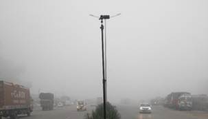
Fig. 1. Data collection setup and snapshot of video data

Tab. 1

Traffic data collection locations

S. No	Name of the road	Location of the section	Lanes per carriageway	Type of road
1	NH-16, (Chennai-Kolkata Highway)	Salkia, Dist. Howrah West Bengal	3	Urban
2	West Bengal SH-13 (Delhi Road)	Chandannagar, Dist. Hoogly, West Bengal	2	Inter-urban
3	NH-5 (Airport Road)	Knowledge City, Dist. SAS Nagar, Punjab	3	Urban
4	NH-7(Chandigarh-Patiala Road)	Ramgarh, Dist. SAS Nagar, Punjab	2	Urban
5	NH-7 (Rajpura bypass)	Rajpura, Dist. Patiala, Punjab	2	Inter-urban
6	NH-8 (Ambala-Chandigarh Road)	Zirakpur, Dist. SAS Nagar, Punjab	2	Inter-urban
7	NH-44 (Grand Trunk Road)	Rajpura, Dist. Patiala, Punjab	3	Inter-urban
8	NH-44, (Grand Trunk Road)	Madhopur, Dist. Fatehgarh-Sahib, Punjab	3	Inter-urban

Vehicle detection and tracking were conducted by custom-training a machine-learning YOLO algorithm with annotated images from recorded traffic videos [38, 39]. The model achieved mean-average-precision rates (mAP) of detection of 79%, 97%, 82%, 67%, 88% and 50% for buses, cars, trucks, LCVs, two-wheelers, and three-wheelers, respectively. Image trajectories were extracted by combining the detection with the Deep-SORT tracking algorithm, which were then transformed into real-world coordinates using camera calibration [40].

3.2. Smoothing of vehicle trajectory

Vehicle trajectories extracted from video data are prone to noise and can lead to unrealistic kinematic properties [41]. For vehicle trajectories to be both realistic and beneficial, they must exhibit internal, platoon, and physical consistency. Internal consistency ensures that a vehicle's trajectory conforms to the equation of motion [42]. Platoon consistency validates car-following behavior, while physical consistency addresses practical traffic operations [43]. However, a good smoothing technique must consider internal consistency during the smoothing process [41]. A more recent method, Locally Weighted Polynomial Regression (LWPR), is used in this study to smooth the vehicle trajectories [44]. LWPR applies a lower-degree polynomial fitted to localized observations using non-parametric regression, with optimal parameters (window size and polynomial order) determined by minimizing the standard deviation of the mean-squared error (MSE). The smoothing process resulted in a mean-average error (MAE) of 0.103m and a root-mean-squared error (RMSE) of 0.135m for vehicle coordinates. Internal consistency analysis showed minimal discrepancies of 0.06m in position and 0.117m/s in speed. Moreover, speeds and accelerations, derived from smoothed trajectories, were compared to the in‐vehicle GPS measurements over multiple test runs. Statistical tests confirmed similarity (p-value < 0.01) and equivalent standard deviations.

Using the smoothed trajectories, every vehicle's instantaneous lateral, and longitudinal speeds, accelerations are calculated by determining the first (speed) and second-order (acceleration) derivatives of trajectory to time. The direction of the road is regarded as longitudinal, while the direction transverse to the road is considered lateral for calculation in this paper.

3.3. Visibility estimation

Visibility is the farthest distance at which a non-reflective black object can be identified against a uniform background. This study uses Hautiere’s method [19], where visibility is the distance at which contrast drops to 5% of its clear-weather value. A black and white object is moved along the road until it is no longer visible in the camera every ten minutes (or when a drastic change in fog is observed) during foggy weather (Fig. 2).

The contrast ration, (Equation-1) was measured at different distances. Actual distance was calculated from image coordinates converted to real-world by camera calibration [40].

(1)

where denotes brightness values for black (b) and white (w) areas in foggy (f) and clear (c) conditions. The distance at which the contrast difference reaches 5% of its value in clear weather conditions () is termed as the visibility and is calculated by interpolating or extrapolating the obtained contrast values at various distances [12]. Visibility ranged from 50-800 m, aligning with meteorological data. Values above 800 m were obtained from weather records and assumed to have negligible traffic impact.

Fig. 2. Estimation of visibility using black and white objects at various distances

4. ANALYSIS

This study investigates the influence of fog-induced reduced visibility on vehicle dynamics, particularly speed and acceleration patterns under following and free-flow conditions. The ‘following’ condition is defined by (i) lateral overlap, (ii) time headway ≤ 4 sec based on Indo-HCM [45], and more conservative thresholds [46], and (iii) speed difference < 10 km/h. All data were merged; however, statistical analysis and effect-size analysis were conducted to justify combining key kinematic parameters – longitudinal and lateral speed, longitudinal and lateral acceleration – from 2-lane and 3-lane roads. While the ANOVA indicated statistically significant differences (p < 0.01) for accelerations, effect size analysis using Cohen’s d and eta-squared (η²) (mentioned in Table 2) revealed that the practical differences between the 2-lane and 3-lane datasets were negligible. Results of this analysis (d = 0.10-0.22 and η² < 0.01) indicate that lane type accounts for less than 1 % of the total variance in each parameter. These negligible practical differences support the statistical equivalence of the two datasets, and therefore this dataset is combined for subsequent analysis.

Tab. 2

Effect size analysis of different dynamic parameters
between two-lane and three-lane roads

Parameter	Mean		Cohen’s d	η²
	Two-lane	Three-lane
Longitudinal speed	76.28	70.60	0.22	0.009
Lateral speed	1.51	1.62	-0.07	0.001
Longitudinal acceleration	1.45	1.87	-0.21	0.009
Lateral acceleration	0.32	0.28	0.09	0.002

4.1. Effect of fog on lateral and longitudinal speed

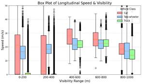
Figure 3 presents a box-plot illustrating the relationship between the obtained speed (longitudinal and lateral) and visibility.

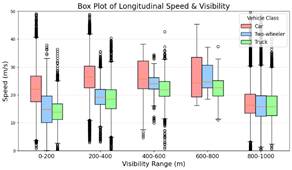
(a) Longitudinal (left) and lateral speed (right) vs. visibility at thefollowing condition

(b) Longitudinal (left) and lateral speed (right) vs. visibility at free-flowing condition

Fig. 3. Box plot of longitudinal and lateral speed at following and free-flowing conditions

Tab. 3

85^th percentile longitudinal and lateral speed of following and free-flowing vehicles

Driving conditions and vehicle type (2W = Two-wheeler)				Fog level (m)
				0-200	200-400	400-600	600-800	Non-foggy
Following vehicles	Longitudinal speed (m/s)	Mean	Car	22.34	26.28	26.14	25.9	17.21
			2W	14.89	19.34	23.41	26.45	16.43
			Truck	14.05	18.28	21.93	22.21	16.38
		85th	Car	29.2	32.25	33.57	34.56	22.92
			2W	21.58	23.86	30.4	32.91	22.62
			Truck	18.51	23.46	26.19	25.96	22.05
	Lateral speed (m/s)	Mean	Car	0.54	0.38	0.47	0.42	0.58
			2W	0.39	0.44	0.21	0.28	0.56
			Truck	0.29	0.27	0.18	0.16	0.47
		85th	Car	1.03	0.67	0.9	0.79	0.89
			2W	0.71	0.77	0.37	0.56	0.77
			Truck	0.49	0.45	0.34	0.32	0.88
Free-flowing vehicles	Longitudinal speed (m/s)	Mean	Car	17.77	13.86	27.24	26.88	18.63
			2W	15.8	18.07	21.8	22.6	17.18
			Truck	3.63	3.71	22.15	22.84	14.83
		85th	Car	32.1	31.68	34.11	37.36	25.12
			2W	22.57	23.79	27.28	32.53	26.6
			Truck	13.72	14.72	26.33	27.17	20.49
	Lateral speed (m/s)	Mean	Car	0.38	0.2	0.38	0.45	0.65
			2W	0.39	0.41	0.27	0.24	0.63
			Truck	0.08	0.06	0.14	0.15	0.41
		85th	Car	0.79	0.48	0.74	0.76	1.11
			2W	0.71	0.69	0.5	0.38	1.27
			Truck	0.16	0.09	0.27	0.28	0.82
Sample size	Following vehicles		Car	978	964	29	20	491
			2W	276	409	9	10	310
			Truck	87	224	119	68	177
	Free-flowing vehicle		Car	3676	1952	71	30	1213
			2W	2043	1282	47	22	945
			Truck	754	688	298	176	598

The 85^th percentile value is used for analysis (Table 3), as it represents the maximum threshold at which most drivers operate, providing a safer benchmark for traffic design and management [47]. Table 3 reveals:

(i) Longitudinal Speed vs. Visibility: As visibility improves, longitudinal speed increases for all vehicles. Surprisingly, car speeds in dense fog remain higher than in clear weather, raising safety concerns.

(ii) Lateral Speed Behavior: Lateral speeds drop in fog, but following cars show slightly higher lateral speeds in dense fog, suggesting reduced lateral stability.

(iii) Risk in Medium Fog: Medium and shallow fog lead to high speeds and poor speed judgment, increasing rear-end collision risk, especially if the lead vehicle brakes suddenly. This trend is consistent with previous literature [8]. The reason was suggested to be the vision loss in the peripheral region due to medium fog. This leads to drivers underestimating their own speeds.

(iv) Truck Driver Behavior: Trucks maintain low speeds in both directions during fog, reflecting consistently safe and cautious driving.

4.2. Effect of fog on lateral and longitudinal acceleration

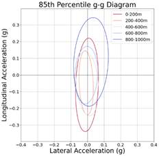
Simultaneous lateral and longitudinal accelerations are visualized using a g-g diagram, where both values are normalized by gravitational acceleration (g) and plotted along horizontal and vertical axes, respectively. This plot, termed the driver capability envelope [48, 49], helps assess dynamic behavior under varying conditions., Fig. 4 presents 85^th percentile g-g envelopes for cars under varying visibility and driving states (following and free-flow), as it is commonly accepted as the breakeven point for such dynamics [49, 50].

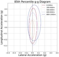
(a) Following cars (b) Free-flowing cars

(a) Following two-wheelers (b) Free-flowing two-wheelers

(a) Following trucks (b) Free-flowing trucks

Fig. 4. g-g diagram of following and free-flowing vehicles in different visibility

The g-g diagram, presented in Fig. 4, is ellipsoidal with the major axis at the longitudinal acceleration end. It shows a narrower spread of lateral acceleration for medium and shallow fog. This suggests that drivers are more cautious in medium and shallow foggy weather and avoid acceleration in any direction. However, in dense fog, the spread increases towards both axes for cars and two-wheelers, suggesting that drivers may be slightly more inclined to lateral and longitudinal movements in dense fog than at other fog levels. The envelope inclines towards the braking side for following cars in fog, indicating frequent and rapid braking action by following vehicles to keep a safe distance from the lead vehicle. For two-wheelers, this envelope inclines toward the accelerating side in clear weather. However, for truck drivers, the envelopes are very small in every fog conditions, especially in free-flow conditions. This suggests that truck drivers drive very stably in foggy weather which is the safest driving behavior.

For a clearer understanding of the acceleration behavior, 85^th percentile values of longitudinal and lateral acceleration are plotted with visibility and shown in Fig. 5, and the discussion follows thereafter.

(i) Longitudinal acceleration (A) and deceleration (D): Fig. 5 shows that longitudinal A/D is high (85^th percentile value >3m/s²) for free-flowing and following vehicles in denser fog for cars and two-wheelers, indicating that the drivers become highly sensitive to acceleration and braking. Further, this abrupt driving decreases as the visibility improves. Values of these parameters are higher for free-flowing cars and two-wheelers in fog, since the free-flowing vehicle is traveling without any guiding element, enabling the drivers to be more restless in their longitudinal movement. However, A/D values are very low for trucks, especially in free-flow conditions, suggesting truck drivers drive very safely in lower visibility, as also observed in their speed behavior.

(ii) Lateral acceleration and deceleration: From Fig. 5, it can be observed that lateral A/D decreases in foggy weather (<1m/s²). For following vehicles, this is likely because, in reduced visibility, drivers focus on following the lead vehicle closely, primarily adjusting their speed through longitudinal acceleration and braking rather than lateral maneuvers. For free-flowing vehicles, no particular trend is observed, although overall lesser lateral A/D values are observed in fog. Similar findings are observed for two-wheelers and trucks, with very low A/D values for trucks.

Overall, it was revealed that car and two-wheeler drivers tend to exhibit more restless longitudinal movements in dense fog. This behavior may result from subtle visual cues caused by the dense fog, which can create the illusion of obstacles or hazards ahead. Such visual misinterpretations often prompt rapid acceleration or deceleration, compromising safety and increasing crash risk. Sudden maneuvers by a leading vehicle in dense fog may leave following vehicles with insufficient time to react, significantly raising the likelihood of collisions. However, truck drivers drive very cautiously in any fog conditions, especially in free-flow conditions.

(a) Longitudinal (left) and lateral (right) acceleration vs. visibility at following vehicle

(b) Longitudinal (left) and lateral (right) acceleration vs. visibility at
free-following vehicle

Fig. 5. Variation of longitudinal and lateral acceleration and deceleration with visibility

5. CONCLUSION

This study investigates the effects of reduced visibility due to fog on vehicle dynamics in weak-lane discipline traffic, focusing on speed, lateral and longitudinal acceleration, and car-following behavior under various fog conditions. The findings of (i) increased longitudinal speed in shallow fog levels, (ii) decreased lateral speed in foggy weather, (iii) more restless longitudinal movement (higher braking/acceleration up to 4 m/s²) by cars and two-wheelers in foggy weather, (iv) lesser lateral acceleration/deceleration values (less than 1m/s²), and (v) safest driving by trucks, in this paper can be detrimental for predicting driving movement in foggy weather. The findings of speed in fog, and lateral and longitudinal acceleration in non-foggy weather confirm with the studied literature [49].

The findings in this paper highlight the need for better traffic management and safety measures to mitigate risks associated with lane-changing and speed variability in dense fog
(0-200 m). Traffic safety measures, such as improved road markings, better lane management, and fog-related warning systems, may be implemented to address these behaviors.

Future research could focus on incorporating these findings into car-following model calibration and traffic simulation models to replicate driver behavior more accurately in foggy conditions. These models could be applied to generate traffic streams under various visibility levels and improve accident analysis, allowing for more effective warning systems that alert drivers about impending hazards caused by reduced visibility.

References

1. Wu Y., M. Abdel-aty, J. Lee. 2018. “Crash risk analysis during fog conditions using real-time traffic data”. Accident Analysis & Prevention 114: 4-11. DOI: 10.1016/j.aap.2017.05.004.

2. Moore R.L., L. Cooper. 1972. Fog and Road Traffic.

3. Edwards J.B. 1999. “Speed adjustment of motorway commuter traffic to inclement weather”. Transportation Research Part F: Traffic Psychology and Behaviour 2: 1-14. DOI: 10.1016/S1369-8478(99)00003-0.

4. Khan M.N., A. Ghasemzadeh, M.M. Ahmed. 2018. “Investigating the impact of fog on freeway speed selection using the SHRP2 naturalistic driving study data”. Transportation Research Record: Journal of the Transportation Research Board 2672(16): 93-104. DOI: 10.1177/0361198118774748.

5. Peng Y., M. Abdel-aty, J. Lee, Y. Zou. 2018. “Analysis of the impact of fog-related reduced visibility on traffic parameters”. Journal of Transportation Engineering, Part A: Systems 144: 1-8. DOI: 10.1061/jtepbs.0000094.

6. Al-Ghamdi A.S. 2007. “Experimental evaluation of fog warning system”. Accident Analysis & Prevention 39: 1065-1072. DOI: 10.1016/j.aap.2005.05.007.

7. Snowden R.J., N. Stimpson, R.A. Ruddle. 1998. “Fog and driving”. Nature 392(450).

8. Pretto P., M. Vidal, A. Chatziastros. 2008. “Why fog increases the perceived speed”. In: Proceedings of the Driving Simulation Conference: 223-235. DSC 2008 Europe – Monaco – 31 January - 1 February 2008.

9. Kim Y.-K., H. Kim, J.-W. Seo, H.-Y. An, Y.-H. Choi. 2017. “Meteorological analysis of the sea fog in winter season on Gyeonggi Bay, Yellow Sea: A case study for the 106-vehicle pileup on February 11, 2015”. Journal of Coastal Research 79: 124-128. DOI: 10.2112/SI79-026.1.

10. Munigety C.R., T.V. Mathew. 2016. “Towards behavioral modeling of drivers in mixed traffic conditions”. Transportation in Developing Economies 2: 1-20. DOI: 10.1007/s40890-016-0012-y.

11. Damani J., P. Vedagiri. 2021. “Safety of motorised two wheelers in mixed traffic conditions: Literature review of risk factors”. Journal of Traffic and Transportation Engineering 8: 35-56. DOI: 10.1016/j.jtte.2020.12.003.

12. Pandit A., A.K. Budhkar. 2025. “Impact of fog levels on free-flow speeds in mixed traffic conditions”. Communications – Scientific Letters of the University of Žilina. DOI: 10.26552/com.C.2025.019.

13. Li Q., H. Yao, X. Li. 2022. “A matched case-control method to model car-following safety”. Transportmetrica A: Transport Science 19(3). DOI: 10.1080/23249935.2022.2055198.

14. Kar P., S.P. Venthuruthiyil, M. Chunchu. 2023. “Assessing the crash risk of mixed traffic on multilane rural highways using a proactive safety approach”. Accident Analysis & Prevention 188: 107099. DOI: 10.1016/j.aap.2023.107099.

15. WMO G. 1996. Guide to Meteorological Instruments and Methods of Observation.

16. Dumont E., V. Cavallo. 2004. “Extended photometric model of fog effects on road vision”. Transportation Research Record: Journal of the Transportation Research Board 1862: 77-81.

17. Ovseník Ľ., J. Turán, P. Mišenčík, J. Bitó, L. Csurgai-Horváth. 2013. “Fog density measuring system”. Acta Electrotechnica et Informatica 12(2): 67-71. DOI: 10.2478/v10198-012-0021-7.

18. Meteorological A. 2013. AMOFSG/10. Forecast Study Group.

19. Hautière N., D. Aubert, E. Dumont. 2007. “Mobilized and mobilizable visibility distances for road visibility in fog”. In: Proceedings of the 26th Session of the International Commission on Illumination (CIE): 1-4. Beijing, China.

20. Cavallo V. 2002. “Perceptual distortions when driving in fog”. In: Proceedings of the Conference on Traffic and Transportation Studies (ICTTS): 965-972.

21. Peng Y., M. Abdel-aty, M. Lee, Y. Zou. 2018. “Analysis of the impact of fog-related reduced visibility on traffic parameters”. Journal of Transportation Engineering, Part A: Systems 144: 1-8. DOI: 10.1061/JTEPBS.0000094.

22. Tu H., Z. Li, H. Li, K. Zhang, L. Sun. 2015. “Driving simulator fidelity and emergency driving behavior”. Transportation Research Record: Journal of the Transportation Research Board 2518: 113-121. DOI: 10.3141/2518-15.

23. Pretto P., M. Vidal, A. Chatziastros. 2008. “Why fog increases the perceived speed”. In: Proceedings of the Driving Simulation Conference: 223-235. DSC 2008 Europe – Monaco – 31 January - 1 February 2008.

24. Kocmond W.C., K. Perchonok. 1970. “Highway fog”. NCHRP Research Results Digest 15.

25. Federal Highway Administration. Mitigation Strategies for Design Exceptions. Available at: https://safety.fhwa.dot.gov/geometric/pubs/mitigationstrategies/chapter3/ 3_stopdistance.cfm.

26. Hoogendoorn R.G., S.P. Hoogendoorn, K.A. Brookhuis, W. Daamen. 2011. “Adaptation longitudinal driving behavior, mental workload, and psycho-spacing models in fog”. Transportation Research Record: Journal of the Transportation Research Board 2249: 20-28. DOI: 10.3141/2249-04.

27. Hoogendoorn R. 2012. Empirical Research and Modeling of Longitudinal Driving Behavior Under Adverse Conditions. Delft, Netherlands: TRAIL Research School.

28. Pei Y., G. Cheng. 2004. “Research on the relationship between discrete character of speed and traffic accident and speed management of freeway”. China Journal of Highway and Transport 17(1): 74-78.

29. Hosseinpour M., A.S. Yahaya, A.F. Sadullah. 2014. “Exploring the effects of roadway characteristics on the frequency and severity of head-on crashes: Case studies from Malaysian Federal Roads”. Accident Analysis & Prevention 62: 209-222. DOI: 10.1016/j.aap.2013.10.001.

30. Chaudhari M. 2020. “Analyzing risky behavior in traffic accidents”. In: Proceedings of the IEEE International Conference on Systems, Man, and Cybernetics (SMC 2020): 464-471. DOI: 10.1109/SMC42975.2020.9283330.

31. Zhao C., H. Yu, T.G. Molnar. 2023. “Safety-critical traffic control by connected automated vehicles”. Transportation Research Part C: Emerging Technologies 154: 104230. DOI: 10.1016/j.trc.2023.104230.

32. Mallikarjuna C., B. Tharun, D. Pal. 2013. “Analysis of the lateral gap maintaining behavior of vehicles in heterogeneous traffic stream”. Procedia – Social and Behavioral Sciences 104: 370-379. DOI: 10.1016/j.sbspro.2013.11.130.

33. Gong B., R. Wei, D. Wu, C. Lin. 2020. “Fleet management for heavy-duty vehicles and connected automated vehicles on highway in dense fog environment”. Journal of Advanced Transportation. Article ID: 8842730. DOI: 10.1155/2020/8842730.

34. Brooks J.O., M.C. Crisler, N. Klein, R. Goodenough, R.W. Beeco, C. Guirl, P.J. Tyler, A. Hilpert, Y. Miller, J. Grygier, et al. 2011. “Speed choice and driving performance in simulated foggy conditions”. Accident Analysis & Prevention 43: 698-705.

35. Zhang Y., Z. Guo, B. Zhu, Z. Fan, H. Zhang. 2021. “Analysis of compensatory driving behavior under fog weather conditions”. Green and Intelligent Technologies for Sustainable and Smart Asphalt Pavements: 662-668. CRC Press.

36. Soria I., L. Elefteriadou, A. Kondyli. 2014. “Assessment of car-following models by driver type and under different traffic and weather conditions using data from an instrumented vehicle”. Simulation Modelling Practice and Theory 40: 208-220.

37. Hammit B.E., A. Ghasemzadeh, R.M. James, M.M. Ahmed, R.K. Young. 2018. “Evaluation of weather-related freeway car-following behavior using the SHRP 2 naturalistic driving study database”. Transportation Research Part F: Traffic Psychology and Behaviour 59: 244-259.

38. Jocher G., A. Chaurasia. 2023. “YOLO by Ultralytics (Version 8.0.0)”. Computer software. Available at: https://github.com/ultralytics/ultralytics.

39. Tao J., H. Wang, X. Zhang, X. Li, H. Yang. 2017. “An object detection system based on YOLO in traffic scene”. In: Proceedings of the 6th International Conference on Computer Science and Network Technology (ICCSNT 2017): 1532-1536. IEEE.

40. Fung G.S.K., N.H.C. Yung, G.K.H. Pang. 2003. “Camera calibration from road lane markings”. Optical Engineering 42: 2967. DOI: 10.1117/1.1606458.

41. Venthuruthiyil S.P., M. Chunchu. 2018. “Trajectory reconstruction using locally weighted regression: A new methodology to identify the optimum window size and polynomial order”. Transportmetrica A: Transport Science 14: 881-900. DOI: 10.1080/23249935.2018.1449032.

42. Kanagaraj V., G. Asaithambi, T. Toledo, T.C. Lee. 2015. “Trajectory data and flow characteristics of mixed traffic”. Transportation Research Record: Journal of the Transportation Research Board 2491: 1-11. DOI: 10.3141/2491-01.

43. Punzo V., D.J. Formisano, V. Torrieri. 2005. “Nonstationary Kalman filter for estimation of accurate and consistent car-following data”. Transportation Research Record: Journal of the Transportation Research Board 1934(1): 3-12. DOI: 10.1177/0361198105193400101.

44. Jekabsons G. 2016. Locally weighted polynomials toolbox for MATLAB/Octave. Riga, Latvia: Available at http://www.cs.rtu.lv/jekabsons.

45. Indian Highway Capacity Manual: Indo-HCM. 2017. CSIR.

46. Toledo T., H.N. Koutsopoulos, M. Ben-Akiva. 2007. “Integrated driving behavior modeling”. Transportation Research Part C: Emerging Technologies 15: 96-112. DOI: 10.1016/j.trc.2007.02.002.

47. White L. 2011. Modeling of 85th Percentile Speed for Rural Highways for Enhanced Traffic Safety: Final Report – FHWA-OK-11-07 (January 2009): 1-25.

48. Biral F., M. Da Lio, E. Bertolazzi. 2005. “Combining safety margins and user preferences into a driving criterion for optimal control-based computation of reference maneuvers for an ADAS of the next generation”. In: Proceedings of the IEEE Intelligent Vehicles Symposium: 36-41. DOI: 10.1109/IVS.2005.1505074.

49. Mahapatra G., A.K. Maurya. 2018. “Dynamic parameters of vehicles under heterogeneous traffic stream with non-lane discipline: An experimental study”. Journal of Traffic and Transportation Engineering 5: 386-405. DOI: 10.1016/j.jtte.2018.01.003.

50. Xu J., W. Lin, X. Wang, Y.M. Shao. 2017. “Acceleration and deceleration calibration of operating speed prediction models for two-lane mountain highways”. Journal of Transportation Engineering 143: 1-13. DOI: 10.1061/JTEPBS.0000050.

Received 04.06.2025; accepted in revised form 20.08.2025

Scientific Journal of Silesian University of Technology. Series Transport is licensed under a Creative Commons Attribution 4.0 International License

---

[1] Department of Civil Engineering, Indian Institute of Engineering Science and Technology, Shibpur, Howrah, India. Email: pandit.angshuman333@gmail.com. ORCID: https://orcid.org/0000-0002-1074-0067

[2] Department of Civil Engineering, Indian Institute of Engineering Science and Technology, Shibpur, Howrah, India. Email: anujbudhkar@gmail.com. ORCID: https://orcid.org/0000-0002-5931-806X