Article
citation information:
Khorshidi, N., Afandizadeh Zargari, S., Mirzahossein, H., Heidari, H.,
Waller, T. Predicting travel-time reliability in road networks: a Fitrnet-based approach – a case study of England. Scientific Journal of Silesian University of
Technology. Series Transport. 2025, 126,
79-95. ISSN: 0209-3324. DOI: https://doi.org/10.20858/sjsutst.2025.126.5.
Navid KHORSHIDI[1], Shahriar AFANDIZADEH ZARGARI[2],
Hamid MIRZAHOSSEIN[3], Hanif HEIDARI[4],
Travis WALLER[5]
PREDICTING
TRAVEL-TIME RELIABILITY IN ROAD NETWORKS: A FITRNET-BASED
APPROACH – A CASE STUDY OF ENGLAND
Summary. This Travel Time
Reliability (TTR) is a crucial aspect of
transportation planning and management. It affects individual decisions,
scheduling, and productivity, and has significant financial implications for
passengers and goods. Traffic congestion is a major factor impacting TTR, which can be classified as recurring (predictable) or
non-recurring (unanticipated). Researchers have developed various definitions
and measures for TTR and Planning Time Index (PTI) is one of these indexes. Proper communication of TTR is essential, and numerical measures like PTI are commonly used to convey this information to travelers. Machine Learning (ML) models, particularly
neural networks, have become increasingly popular for TTR
estimation due to their ability to handle complex relationships and
high-dimensional data. This study proposes using Fitrnet,
a feedforward fully connected neural network, for predicting TTR at a network level. While Fitrnet
has been used in other fields of engineering, its application in TTR estimation is novel. The study uses a dataset from the
UK government covering the Strategic Road Network from April 2015 to March
2021. Results show that a Fitrnet model with 5 hidden
layers can accurately predict PTI, with MAPE values below 10% in most cases, demonstrating the
effectiveness of Fitrnet for TTR
prediction in smaller datasets. The study contributes to the growing body of
research on TTR modeling by
proposing a new approach using Fitrnet and applying
it to a previously unused dataset.
Keywords: Travel Time Reliability (TTR),
Fitrnet machine learning algorithm, England's
Strategic Road Network (SRN), prediction accuracy
1. INTRODUCTION
Travel Time Reliability (TTR)
is a fundamental component of transportation planning and management. Its
significance stems from the impact on various aspects of transportation
systems, particularly those influenced by temporal variations in travel time,
also known as TTR. TTR
affects individual decisions, scheduling, and productivity, and has significant
financial implications for passengers and goods [1].
Studies have confirmed that traffic congestion
is a critical factor that makes travel time unreliable. Traffic congestion can
be classified as recurring and non-recurring congestion. Recurring congestion
is predictable and often occurs when the demand for using a facility exceeds
its capacity. On the other hand, non-recurring congestion temporarily reduces
the capacity of transportation systems and is usually unexpected [2].
Researchers have used a wide range of
definitions for TTR, but since it is out of the scope
of this paper, they will be mentioned herein briefly. The first definition
attempts were made by Polus and Schofer in 1979,
defining operational consistency as reliability [3]. According to the Texas Transportation
Institute, TTR is the dependability of travel time as
measured across different times of day or from day to day [4]. Also, Shaw summarized three of the most
frequently used reliability definitions in his study, and only one of them is
mentioned herein: the variability between the expected travel time and the
actual travel time [5]. Based on this definition, numerical
measures were extracted to estimate TTR, including PTI and Travel Time Index (TTI).
Further information on PTI, which is used as the
measure of this study, will be provided in the subsequent paragraphs. According
to Kuhn et al., PTI is defined as the ratio of the 95th
percent peak period travel time to the free flow travel time. Also, TTI can be defined as the ratio of average travel time in
peak hours to free-flow travel time. It should be noted that both the PTI and TTI are unitless measures [6].
Conveying (TTR)
properly is as crucial as defining it, as accurate information transfer is
necessary for travelers to comprehend it. To provide a reliable tool for
communicating with TTR, experts suggested using
numerical measures such as PTI, TTI,
Buffer Index (BI), and so on. Detailed explanations of these measures are
available in the “Lexicon for conveying travel time reliability information”[6] and “Incorporating reliability performance
measures into operations and planning modeling tools” [7]. In this study, PTI is used for the sake of modeling. Numerous advantages,
including the ability to be compared with TTI
directly, capturing extreme variations, and its practical application have made
this measure a valuable tool for modeling TTR [8].
TTR is a widespread concept in transportation, and
researchers have considered its application in various aspects of their
research. The first class of studies aims to estimate TTR
in links or networks. TTR has also proved itself as
an influential factor in the traffic assignment process [9], controlling and improving the performance
of intersections [10], and route choice behavior [11]. While this study contributes to the body
of research on TTR, it aligns with the growing
interest in this area.
Today, accurate estimation of TTR has gained attention. Accurate forecasting of TTR is essential to both transportation authorities and
road users. This importance served as a motivation for developing suitable
tools that could be beneficial.
Single distribution modeling techniques were
among the first and the most widely used methods for predicting TTR [9]. Researchers utilized Normal, Lognormal,
Gamma, Burr, and Generalized Extreme Value (GEV) distributions to address the
problem of TTR estimation. Lomax and Margiotta followed a normal distribution as a part of their
modeling approach [12]. Also, lognormal distribution
was utilized by Emam and Al-Deek
in modeling TTR of I-4 corridor in, Florida, US
[13]. In a study conducted by Polus, an
inference was made about the application of Gamma distribution in modeling TTR [14]. In a work published by Taylor, the practical use
of Burr distribution in modeling TTR was evaluated
[15]. Finally, Generalized Extreme Value (GEV) could prove itself as a promising
tool for modeling TTR in the publication of Zhang et
al. [16]. Due to multimodal distribution of travel time, which is a consequence
of traffic congestion in urban transportation systems, single distribution
models failed to represent a promising performance; hence, mixture distribution
models were introduced. Mixture models comprise a weighted combination of
single distribution models. Guo et al. proposed a
multi-state approach for modeling TTR. They utilized
discrete travel time states to report and forecast reliability based on
probabilities between these states [17]. On the other hand, Rahmani
et al. developed a non-parametric approach. Their methodology could estimate
route travel time distributions from low-frequency floating car data [18]. Finally,
Chen et al. developed a copula-based approach to estimate TTR
on urban arterials by considering the dependence structure between segments of
a road for better estimation of travel time distributions [19].
The ability of regression models to predict continuous
variables, along with simplicity, efficiency, interpretability, and
generalizability have made them a popular tool for modeling [20]. Researchers in the field of TTR modeling have also used it widely. Elefteriadou
and Cuy collected data on a roadway in Philadelphia
and used congestion, weather conditions, work zones, and crashes as independent
variables, to estimate a linear regression model for predicting TTR [21]. Charlotte and Sandra presented innovative
regression-based explanatory models for understanding variability in road
travel times, aiming to incorporate reliability benefits into transport projects
[22]. Kwon et al. developed their empirical modeling approach for predicting TTR along freeway sections by considering five key
components: incidents, weather, work zones, special events, and inadequate base
capacity or bottlenecks. Their method leveraged quantile regression [23]. Also,
Zheng et al. focused on a corridor in China and developed a linear
regression model to explain the relationship between travel time and its
reliability, standard deviation, skewness, and other relevant traffic characteristics
[24].
Whereas regression models have benefits, ML
methods are often preferred over regression models for many reasons, including
handling nonlinear relationships, high-dimensional data, robustness to
outliers, and feature interactions and importance. Gradually, Machine Learning
(ML) models became practical and were used as reliable tools in various fields
of transportation engineering, including TTR
estimation. Since this study utilizes Fitrnet, a
feedforward fully connected neural network for regression, studies with ML as
their methodology will be further analyzed. Table 1 describes studies that have
used ML techniques as their methodology. The relevant data is too detailed and
complicated to be described thoroughly in a table, so the interested reader is
referred to cited articles for further information.
It should be noted that the number of studies
that focus on Travel Time Prediction (TTP) is much
more than articles considering TTR estimation. It is
thought that TTP and TTR
imply the same concept, whereas they represent two distinct concepts in
transportation engineering. In better words, they are related, but TTP offers an estimate of the required time for a trip from
point A to point B, whereas TTR prediction estimates
how consistent those travel times are.
This study focuses on developing a Fitrnet method for predicting TTR
at a network level. To the best of our knowledge, Fitrnet
has been used in only 43 studies in Google Scholar, primarily in other fields
of engineering. Its usage in traffic and transportation engineering has been
limited, with only one study focusing on the electrification of transportation,
and was not previously used for TTR estimation. Table
2 will provide information on studies that have utilized Fitrnet
as their methodology and highlights their scope.
Tab. 1
Summary of conducted studies in TTR estimation
|
Author(s) |
Type of network/Link |
Methodology |
|
Zhang et al. [25] |
Interstate segments in Virginia |
Quantile regression |
|
Zhang and Chen [26] |
Interstates 71 and 75 in Kentucky |
Decision tree and Quantile regression |
|
Zhang et al. [27] |
Interstate segments in Virginia |
Quantile
regression Random
Forest Regression |
|
Babiceanu and Lahiri [28] |
Interstate segments in Virginia |
Classification and Regression Trees |
|
Wu et al. [29] |
Urban arterial in Texas |
Feedforward Neural Network |
|
Zhao et al. [30] |
Interstate segments in Virginia |
Quantile Random
Forests (QRF) Generalized Random
Forests (GRF) |
|
Li et al. [31] |
Urban road network in
China |
Long Short-Term Memory
(LSTM) Quantile Regression |
Tab. 2
Summary of some of the studies utilizing Fitrnet as their modeling tool
|
Author(s) |
Field of study |
Author(s) |
Field of study |
|
Sennefelder et al. [32] |
Electrification of transportation |
Oh et al. [33] |
Applied thermal engineering |
|
Shahbazi et al. [34] |
Thermal modeling |
Cousins et al. [35] |
Bioenergy |
As such, this paper adds the following to the
previous body of research on TTR:
·
Proposes Fitrnet approach to analyze TTR at the network level
Also, it is worth noting that the dataset
utilized in this study has been used six times previously. In Table 3, a
summary of these studies is provided. None of them were related to modeling TTR.
Tab. 3
Summary of studies utilizing the dataset of this study
|
Author(s) |
Focus of study |
Methodology |
|
De Gan et al. [36] |
Air pollution |
Accurate simulation of
traffic-related air pollution |
|
Hadjidemetriou et al. [37] |
Transport planning |
Adaptive policy
pathways used in flood-risk planning |
|
Greenhalgh et al. [38] |
Urban Planning |
Temporal and
statistical analysis, GIS |
|
O'Garra& Fouquet [39] |
Ecological economics |
Regression analysis |
|
Gorbunov et al. [40] |
Travel time |
Statistical analysis |
|
Oakley [41] |
Transport infrastructure |
Analytical report/ No methodologies |
As Table 3 suggests, none of the previous
studies utilizing this dataset has focused on predicting TTR,
so it is the first time this data is being used for this purpose.
The remainder of this paper is organized as
follows: Section 2 introduces the methods, including the dataset used in model
development and the technique employed to predict TTR.
Section 3 analyzes results relevant to network-level predictions. Finally,
Section 4 concludes the paper.
2. METHODS
It is acknowledged that using ML, and
especially neural networks, is well-documented in transportation engineering.
It should be noted that the specific use of Fitrnet
has not been mentioned either in TTR prediction or
other transportation-related studies.
The Fitrnet function
is used to establish a feed-forward neural network. This kind of network is
structured in layers, with each layer consisting of several neurons or nodes.
Data in this network flows from the input layer straight to the output layer,
without any circular paths, which is why it's referred to as 'feed-forward'.
The most appropriate reference that provides
information about the Fitrnet is the official
documentation of MATLAB. This document can be
accessed via MathWorks’ website[6]. In the Fitrnet,
there is a connection between network input, which is known as predictor data,
and the first layer of the neural network, which is fully connected. Also,
there are connections between subsequent layers and previous layers. Those as
mentioned earlier, fully connected layers take the input and multiply them by a
weight matrix. In the next step, a bias vector is added. Each fully connected
layer, except for the last one, is followed by an activation function. Finally,
predicted response values, which are the final fully connected layers, produce
the network’s output.
To better realize how Fitrnet
works, each part is broken down to represent its basic usage. First, the model
should be initialized. The next step is the optimization of hyperparameters,
which is optional and is out of the scope of this article (a brief explanation
about all of them is mentioned). Then, the neural network has to be trained.
This process is vital, as the network learns to generalize input-output mapping
without memorization. Cross-validation can also be performed during the training
process. After training the model, its performance should be evaluated using
the loss function. This function could be either Mean Squared Error (MSE), Root Mean Squared Error (RMSE),
Mean Absolute Percentage Error (MAPE), or other
proper measures. It should be noted that RMSE
measures the average difference between values predicted by a model and the
actual values, whereas MAPE measures the average
magnitude of error produced by a model, Finally,
the trained model is used to make predictions on new data. As explained, the
steps for developing a Fitrnet model are similar to
those for other machine learning models, with the primary difference being the
unique structure of the Fitrnet model itself.
The hyperparameters
of Fitrnet in MATLAB are as
follows:
· Layer
size: The size of the layer dictates the quantity of fully interconnected
layers within the neural network. Fitrnet adjusts the size of each layer within
a range of 1 to 300. Typically, Fitrnet optimizes across three fully
interconnected layers, not including the last fully interconnected layer.
· Activation:
This hyperparameter determines the activation function for every fully
connected layer in the neural network, except for the last one. The Fitrnet
method optimizes over a set that includes 'relu', 'tanh', 'sigmoid', and
'none'. The role of an activation function is to add non-linearity to the
model, which enables it to identify and learn more intricate patterns in the
data.
· Lambda:
This hyperparameter, known as Lambda, influences the intensity of the
regularization component in the loss function. Regularization is a method
employed to avoid overfitting by incorporating a penalty term into the loss
function. The Lambda hyperparameter is responsible for setting the size of this
penalty term. Fitrnet fine-tunes Lambda across a continuous range from 1e-5 to
1e5.
· Standardize:
The "Standardize" hyperparameter is a boolean value that determines
if the predictor data should be standardized. When set to true, it adjusts each
numeric predictor variable based on its respective column mean and standard
deviation, effectively centering and scaling them. This process of
standardization ensures that the model is not affected by the different scales
used for the predictor measurements.
· Layer
weights initializer: The layer weights initializer is a hyperparameter that
decides the method used to set the weights for each fully connected layer.
Fitrnet adjusts the layer weights initializer among the options 'glorot' and
'he'. The 'glorot' initializer selects from a uniform distribution with a mean
of zero and a variance of ![]() , where I
represents the input size and O is the output size of the layer. On the other
hand, the 'he' initializer selects from a normal distribution with a mean of
zero and a variance of
, where I
represents the input size and O is the output size of the layer. On the other
hand, the 'he' initializer selects from a normal distribution with a mean of
zero and a variance of ![]() , where I is the
input size of the layer.
, where I is the
input size of the layer.
· Layer
biases initializer: The layer biases initializer is a hyperparameter that sets
the starting values for the biases in every fully connected layer. The Fitrnet
algorithm adjusts the layer biases initializer among the options 'zeros' and
'ones'. When 'zeros' are selected, the initial bias for each fully connected
layer is set to 0. If 'ones' is selected, the initial bias for each fully
connected layer is set to 1.
Fitrnet has some benefits, including but
not limited to flexibility in model architecture, standardization of
predictors, automatic initialization of weights and biases, and so on. For
further information on the application of Fitrnet,
the interested reader is referred to the studies mentioned in Table 2.
The utilized dataset of this study includes
data on TTR and is accessible through statistical
datasets of the United Kingdom (UK) government[7] . Table 4 describes the utilized
data, and Figure 1 depicts the distribution of the Strategic Road Network of
England[8].
Tab. 4
Description of utilized data in this study, PTI, average speed, and
average delay
|
Variable |
Number |
Mean |
SD |
Min |
Q1 |
Median |
Q3 |
Max |
|
PTI |
72 |
1.62 |
0.14 |
1.22 |
1.62 |
1.67 |
1.69 |
1.78 |
Before going through the results
section, a concise overview of the dataset is necessary. The data and
statistics of road congestion and travel times on the Strategic Road Network
(SRN) and local 'A' roads can be accessed publicly, including statistics
released by the UK government related to road congestion and reliability. The utilized
database of this study consists of a continuous variable, the TTR metric (PTI). The aggregation
level of records is monthly, spanning from April 2015 to March 2021. PTI represents reliability. To calculate PTI, according to [6], the 95th percentile of travel time
should be divided into free-flow travel time. Free-flow travel times are based
on speed limits for individual road sections. The calculated PTI is on the Strategic Road Network (SRN) level. To do so,
the average of PTI across individual road sections
was calculated, weighting by traffic flows for each section. Moreover, only car
travel time observations were used for calculating PTI.
The behavior of the variable is
shown in Figure 2. The vertical axis labels the values of the variables and the
horizontal axis, labeled “Index”, starts from 0 indicating April 2015 to 72
indicating March 2021 (one unit in the horizontal axis is equivalent to one
month.
The process of creating a Fitrnet model for the database in MATLAB
has been mentioned previously. It should be noted that the data is split into
training and test sets, with 80% of data for training and 20% for testing.
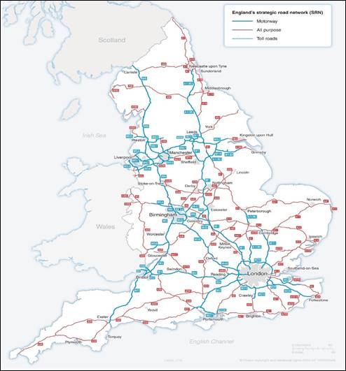
Fig. 1. Spatial distribution of the
Strategic Road Network (SRN) across England
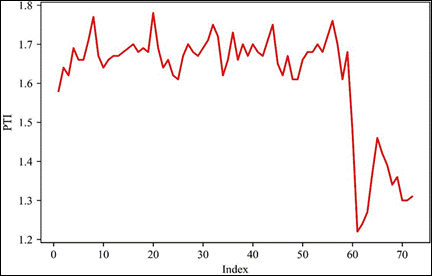
Fig. 2. Analyzing the behavior of PTI as a time series
3. RESULTS
In this section, the results of
developing a Fitrnet model for the described dataset
will be further discussed. First, the evaluation metric used to assess the
performance of the proposed model is reported. This study uses MAPE to determine the model's performance.
To analyze and model the TTR data, the authors used different variants of the Fitrnet model to arrive at the best possible implementation
results. The experimental results show that a feedforward neural network with 5
hidden layers is suitable for predicting PTI. The
model was tested with different train dataset sizes (23, 30, and 37 elements)
to predict the next 3 PTI elements. To show the
stability and robustness of the method, a rolling time window with 5 elements
is considered in all examples. The results are depicted in Figures 3, 4, and 5
for 23, 30, and 37 train dataset sizes respectively. In these plots, the blue
points (blue lines) show actual data, the green points show simulated data and
the red points show predicted data.
In Figure 3, the subfigure 3-D-8
does not generate acceptable results, while other subfigures are approximately
acceptable. The related errors are given in Table 5. The related values of MAPE for Figures 4 and 5 are given in Tables 6 and 7 respectively.
A comparison between Table 3 to Table 5 shows that considering a large enough
training dataset, the proposed model can predict PTI
accurately. Based on our experiments, the considered training dataset size (37)
is appropriate. Increasing the training dataset size is not suggested, since
overfitting may occur. In Figure 5, the subfigures 50-D-2 and 50-D-3 confirm
that overfitting does not occur, while increasing the number of points affects
the error and can bring about overfitting.
Tab. 5
The MAPE for predicting the next three PTIs where 23 elements are used
for training
|
Subfigure (30) |
D-1 |
D-2 |
D-3 |
D-4 |
D-5 |
D-6 |
D-7 |
D-8 |
D-9 |
D-10 |
|
MAPE (%) |
2.78 |
2.61 |
3.86 |
2.38 |
2.66 |
1.14 |
5.23 |
27.95 |
11.10 |
3.96 |
Tab. 6
The MAPE for predicting the next three PTIs where 30 elements are used
for training
|
Subfigure (40) |
D-1 |
D-2 |
D-3 |
D-4 |
D-5 |
D-6 |
D-7 |
D-8 |
|
MAPE (%) |
4.39 |
4.84 |
1.83 |
1.94 |
2.60 |
3.43 |
8.98 |
2.75 |
Tab. 7
The MAPE for predicting the next three PTIs where 37 elements are used
for training
|
Subfigure (50) |
D-1 |
D-2 |
D-3 |
D-4 |
D-5 |
D-6 |
|
MAPE (%) |
1.57 |
3.42 |
1.60 |
0.54 |
4.63 |
8.23 |
To assess the performance of Fitrnet, the authors propose a set of numerical rages to
interpret MAPE as follows:
· 0% <
MAPE < 10%: It is widely considered a highly
precise prediction method. In numerous sectors, a MAPE value below 10% is often
seen as a sign of a strong and reliable model.
· 10%
≤ MAPE < 20%: This range is normally noticed as satisfactory and
suitable for the majority of practical prediction models, particularly in
situations where a certain degree of fluctuation is anticipated.
· 20%
≤ MAPE < 5%: This range might be acceptable
depending on the situation, but it suggests a certain degree of inaccuracy and
implies that the forecasting method could potentially be enhanced.
Based on the values of Table 5 to
Table 7, only in two scenarios (out of 24 scenarios), the MAPE
value exceeded 10, in 30-D-8 and 30-D-9. In the other 22 cases, the MAPE values are below 10%, showing a highly precise and
accurate prediction. This confirms that Fitrnet is a
perfect tool for predicting the reliability of travel time in small datasets.
4. CONCLUSION AND DISCUSSION
TTR is an important aspect of
transportation planning and decision-making, and precise prediction of TTR can support effective transportation planning, route
optimization, and traffic management. Because of their ability to model
complicated, non-linear connections and handle massive, high-dimensional
datasets, many Machine Learning (ML) algorithms have been widely employed to
forecast TTR. Various ML models have been employed
for this purpose, but Fitrnet had not been employed
for this purpose by any earlier study, to the best of the authors' knowledge.
To that end, this research aimed to analyze the prediction performance of Fitrnet by using Strategic Road Network (SRN) level data
from England over 72 months.
We employed multiple iterations of
the Fitrnet model to investigate and simulate travel
time reliability data, ultimately identifying the most effective configuration.
Our findings revealed that a feedforward neural network comprising five hidden
layers demonstrated exceptional proficiency in forecasting Predicted Travel
Time (PTI). To assess the model's consistency and
robustness, we conducted experiments using three distinct training dataset sizes
– 23, 30, and 37 items – to predict the subsequent three PTI
elements. A rolling time window encompassing five consecutive data points was
implemented in each scenario to showcase the method's stability. The results,
presented in Tables 3, 4, and 5, demonstrated the model's accuracy in PTI prediction, with the 37-item dataset proving optimal.
Notably, the low Mean Absolute Percentage Error (MAPE)
values, aside from two exceptional cases, underscored the promising predictive
performance of the proposed model, validating its applicability. Furthermore,
the researchers cautioned against increasing the training dataset size beyond
37 items, as it may lead to overfitting, highlighting the delicate balance
between model complexity and data sufficiency in achieving accurate
predictions. In terms of numerical comparison, this study could achieve the MAPE minimum value of 1.14% in first scenario and in 92% of
cases (22 of 24), the values of MAPE were less than
10%, hence considered high precise prediction. The other studies utilizing Fitrnet could not achieve this level of accuracy, such that
Cousins et al. stated that the minimum value of RMSE
utilizing Fitrnet in their work was almost 5%. The
same statement was mentioned by Sennefelder
et al., but in their work, the values of MAPE
was reported to be 3.6%, larger than minimum value of MAPE
in our work. Finally, in the paper of Shahbazi et
al., the authors could achieve errors less than 1%.
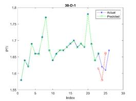
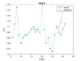
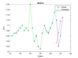
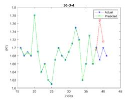
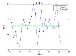
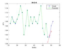
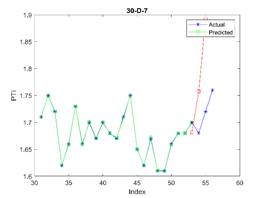
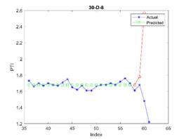
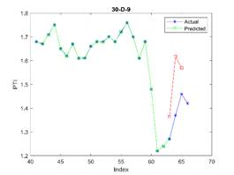
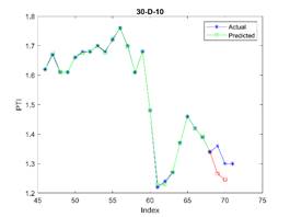
Fig. 3. The actual (blue stars),
simulated (green circle), and predicted (red square) PTI
values in different periods where the first 23 elements are used for training
the model
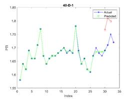
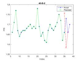
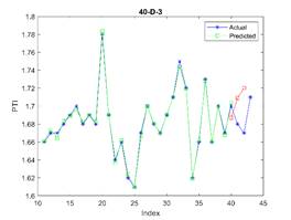
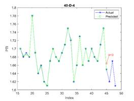
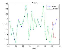
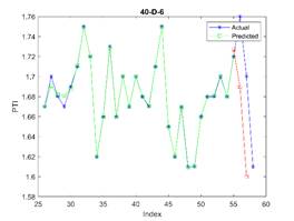
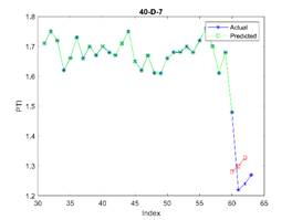
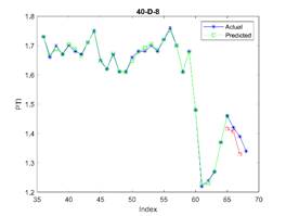
Fig. 4. The actual (blue stars),
simulated (green circle), and predicted (red square) PTI
values in different periods where the first 23 elements are used for training
the model
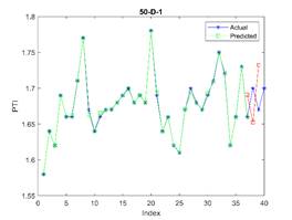
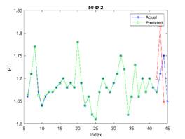
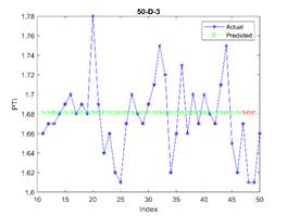
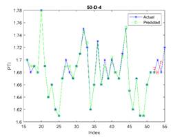
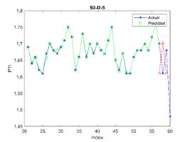
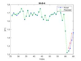
Fig. 5. The actual (blue stars),
simulated (green circle), and predicted (red square) PTI
values in different periods where the first 37 elements are used for training
the model
As future research, this study
proposes two broad ideas that can be considered. The first one is the
application of methods like Genetic Algorithm (GA) that can be used for hyperparameter tuning. As analyzed by researchers, the
values of hyperparameters are set before the learning
process begins. In this study, many of these hyperparameters
were set to the default values, which might change the occurring results.
Furthermore, enriching the dataset can effectively address concerns regarding
its size.
References
1. National Academies of Sciences, Medicine
(US)., Division on Engineering, Physical Sciences, Medicine Division, Division
of Behavioral, Social Sciences, Computer Science, Telecommunications Board, Board
on Health Care Services and Committee on National Statistics. 2022. “Evaluating
Alternative Operations Strategies to Improve Travel Time Reliability”. Transportation
Research Board.
2. TavasoliHojati A., L. Ferreira, S. Washington, P. Charles, A. Shobeirinejad.
2016. “Modelling the impact of traffic incidents on travel time reliability”. Transportation
research part C: emerging technologies. 65: 49-60. DOI:
10.1016/j.trc.2016.06.013.
3. Polus A., J.L. Shofer. 1976. “Analytical study of freeway reliability”. Transportation
Engineering Journal of ASCE 102(4): 857-870. DOI: 10.1061/TPEJAN.0000606.
4. Systematics C. 2005. “Traffic Congestion and
Reliability: Trends and Advanced Strategies for Congestion Mitigation”. No. FHWA-HOP-05-064. United States. Federal Highway
Administration.
5. Shaw T. 2003. “Performance measures of
operational effectiveness for highway segments and systems”. Transportation
Research Board.
6. Kuhn B., L. Higgins, A. Nelson, M. Finely,
G. Ullman, S. Chrysler, K. Wunderlich, V. Shah,
C. Dudek. 2014. “Lexicon for conveying travel time
reliability information”. Transportation
Research Board.
7. Mahmassani H.S., J. Kim, T. Hou, A. Talebpour, Y. Stogios, A. Brijmohan, P. Vovsha. 2014.
“Incorporating reliability performance measures into operations and planning
modeling tools”. Transportation Research Board.
8. Wakabayashi H. 2011. “Travel time
reliability indices for highway users and operators”. In: Network
Reliability in Practice: Selected Papers from the Fourth International
Symposium on Transportation Network Reliability. Springer. DOI: 10.1007/978-1-4614-0947-2_6
9. Zang Z., X. Xu, K. Qu, R. Chen, A. Chen.
2022. “Travel time reliability in transportation
networks: A review of methodological developments”. Transportation Research Part C: Emerging Technologies 143: 103866. DOI: 10.1016/j.trc.2022.103866.
10. Hang J., X. Zhou, J.
Wang. 2020. “Modeling Traffic Function Reliability of Signalized Intersections
with Control Delay”. Advances in Civil Engineering 2020: 1-13. DOI: 10.1155/2020/8894281.
11. Zhu Z., A. Mardan,
S. Zhu, H. Yang. 2021. “Capturing the interaction between travel time
reliability and route choice behavior based on the generalized Bayesian traffic
model”. Transportation research part B: methodological 143: 48-64. DOI: 10.1016/j.trb.2020.11.005.
12. Lomax T., D. Schrank,
S. Turner, R. Margiotta. 2003. “Selecting travel
reliability measures”. Available at:
https://citeseerx.ist.psu.edu/document?repid=rep1&type=pdf&doi=95392d6a899f71fd219751a3e3bd92f4ae13805c.
13. Emam E.B., H. Al-Deek. 2006. “Using real-life dual-loop
detector data to develop new methodology for estimating freeway travel time
reliability”. Transportation research record 1959(1): 140-150. DOI: 10.1177/0361198106195900116.
14. Polus A. 1979. “A study of travel time and
reliability on arterial routes”. Transportation 8(2): 141-151. DOI: 10.1007/BF00167196.
15. Taylor M.A. 2017. “Fosgerau's
travel time reliability ratio and the Burr distribution”. Transportation
Research Part B: Methodological 97: 50-63. DOI: 10.1016/j.trb.2016.12.001.
16. Zhang Z., Q. He, J. Gou, X. Li. 2019.
“Analyzing travel time reliability and its influential factors of emergency
vehicles with generalized extreme value theory”. Journal of Intelligent
Transportation Systems 23(1): 1-11. DOI: 10.1080/15472450.2018.1473156.
17. Guo F., H. Rakha, S. Park. 2010. “Multistate model for travel time
reliability”. Transportation research record 2188(1): 46-54. DOI: 10.3141/2188-06.
18. Rahmani M., E. Jenelius, H.N. Koutsopoulos. 2015. “Non-parametric estimation of route
travel time distributions from low-frequency floating car data”. Transportation
Research Part C: Emerging Technologies 58: 343-362. DOI:
10.1016/j.trc.2015.01.015.
19. Chen M., G. Yu, P. Chen, Y. Wang. 2017. “A
copula-based approach for estimating the travel time reliability of urban
arterial”. Transportation Research Part C: Emerging Technologies 82:
1-23. DOI: 10.1016/j.trc.2017.06.007.
20. Harrell F.E., Kl.
Lee, DB. Matcher. 1985. “Regression models for prognostic prediction:
advantages, problems, and suggested solutions”. Cancer treatment reports
69(10): 1071-1077.
21. Elefteriadou L., X.
Cui. 2007. “A framework for defining and estimating travel time reliability’. Transportation
Research Board 86th Annual Meeting. Washington DC, United States. 2007-1-21
to 2007-1-25.
22. Charlotte C., L.M
Helene, B. Sandra. 2017. “Empirical estimation of the variability of travel
time”. Transportation Research Procedia 25: 2769-2783. DOI: 10.1016/j.trpro.2017.05.225.
23. Kwon J., T. Barkley, R. Hranac,
K. Petty, N. Compin. 2011. “Decomposition of travel
time reliability into various sources: incidents, weather, work zones, special
events, and base capacity’. Transportation Research Record 2229(1):
28-33. DOI: 10.3141/2229-04.
24. Zheng F., J. Li, H. VanZuylen,
X. Liu, H. Yang. 2018. “Urban travel time reliability at different traffic
conditions”. Journal of Intelligent Transportation Systems 22(2):
106-120. DOI: 10.1080/15472450.2017.1412829.
25. Zhang X., M. Zhao, J. Appiah, M. Fontaine.
2022. “Prediction of travel time reliability on interstates using linear
quantile mixed models”. Transportation research record 2677(2): 774-791.
DOI: 10.1177/03611981221108380.
26. Zhang X., M. Chen. 2019. “Quantifying the
impact of weather events on travel time and reliability”. Journal of
advanced transportation 2019(1): 8203081. DOI: 10.1155/2019/8203081.
27. Zhang X., Z. Mo, A. justice, F. Michael. 2021.
“Methods to Analyze and Predict Interstate Travel Time Reliability”. Virginia
Transportation Research Council (VTRC). Available
at: https://rosap.ntl.bts.gov/view/dot/57307.
28. Babiceanu S., S. Lahiri. 2022. “Methodology for Predicting MAP-21 Interstate
Travel Time Reliability Measure Target in Virginia”. Transportation Research
Record 2676(8): 253-266. DOI:
10.1177/03611981221083290.
29. Wu Z., L. Rilett, W.
Ren. 2022. “New methodologies for predicting corridor travel time mean and
reliability”. International Journal of Urban Sciences 26(3): 517-540. DOI: 10.1080/12265934.2021.1899844.
30. Zhao, M., X. Zhang, J. Appiah, M. Fontaine.
2024. “Travel Time Reliability Prediction Using Random Forests”. Transportation
Research Record 2678(3): 531-545. DOI: 10.1177/03611981231182146.
31. Li, H., Z. Wamg, X.
Li, H. Wang, Y. Man, J. Shi, “Travel Time Probability Prediction Based on
Constrained LSTM Quantile Regression”. Journal of Advanced Transportation
2023(1): 9910142. DOI: 10.1155/2023/9910142.
32. Sennefelder R.M., R. Martin-Clemente, R. Gonzalez-Carvajal,
D. Trifonov. 2023. “Data Driven Energy Economy
Prediction for Electric City Buses Using Machine Learning”. IEEE Access
11: 97057-97071. DOI: 10.1109/ACCESS.2023.3311895.
33. Oh S., C. Kim, Y. Lee, H. Park, J. Lee, S.
Kim, J. Kim. 2022. “Analysis of the exhaust hydrogen characteristics of
high-compression ratio, ultra-lean, hydrogen spark-ignition engine using
advanced regression algorithms”. Applied Thermal Engineering 215:
119036. DOI: 10.1016/j.applthermaleng.2022.119036.
34. Shahbazi, M., N.A. Smith, M. Marzband, H.R.
Habib. 2023. “A Reliability-Optimized Maximum Power Point Tracking Algorithm
Utilizing Neural Networks for Long-Term Lifetime Prediction for Photovoltaic
Power Converters”. Energies 16(16): 6071. DOI: 10.3390/en16166071.
35. Cousins D.S., W.G.
Otto, A.H. Rony, K.S.
Pedersen, J.E. Aston, D.B.
Hodge. 2022. “Near-infrared spectroscopy can predict anatomical abundance in
corn Stover”. Frontiers in Energy Research 10: 836690. DOI: 10.3389/fenrg.2022.836690.
36. De Gan B.M., M. Loxham, C. Vanderwel. 2022. “Simulation of outdoor air pollution in
Southampton”. Proceedings of the International Conference on Evolving Cities.
DOI: 10.55066/proc-icec.2022.103.
37. Hadjidemetriou G.M., J. Teal, L. Kapetas, A.K. Parlikad. 2021. “Flexible
planning for intercity multimodal transport infrastructure”. Journal of
Infrastructure Systems 28(1): 05021010. DOI:
10.1061/(ASCE)IS.1943-555X.0000664.
38. Greenhalgh P., H.M.
King, K. Muldoon-Smith, J. Ellis. 2021. “The new distribution: Spatio-temporal analysis of large distribution warehouse
premises in England and Wales”. Urban Planning 6(3): 399-414. DOI: 10.17645/up.v6i3.4222.
39. O'Garra T., R.
Fouquet. 2022. “Willingness to reduce travel consumption to support a
low-carbon transition beyond COVID-19”. Ecological
Economics 193: 107297. DOI: 10.1016/j.ecolecon.2021.107297.
40. Gorbunov R.N., Z.V. Gorbunova, V.S. Kolchin, A.Y.
Mikhailov, Z.T. Pirov.2019. “Analysis of the impact of the sample size on
the accuracy of determining the travel time and buffer indices”. IOP Conference Series: Materials Science and
Engineering 632: 012042. DOI: 10.1088/1757-899X/632/1/012042.
41. Oakley M. 2019. “Moving
Forward Together: Delivering the transport infrastructure that businesses
need”. Available at:
https://wpieconomics.com/wp-content/uploads/2019/09/190911_Critical-Infrastructure_Web_Spreads-Final.pdf.
Received 31.07.2024; accepted in revised form 05.11.2024
![]()
Scientific
Journal of Silesian University of Technology. Series Transport is licensed
under a Creative Commons Attribution 4.0 International License