Article citation information:

Budzyński, A., Cieśla, M. Application of a machine learning model for forecasting freight rate in road transport. Scientific Journal of Silesian University of Technology. Series Transport. 2025, 126, 23-48. ISSN: 0209-3324. DOI: https://doi.org/10.20858/sjsutst.2025.126.2.

Artur BUDZYŃSKI[1], Maria CIEŚLA[2]

APPLICATION OF A MACHINE LEARNING MODEL FOR FORECASTING FREIGHT RATE IN ROAD TRANSPORT

Summary. Recent global trends related to the forecasting freight prices is a complex task that involves considering various factors and variables that can affect the pricing dynamics in the sustainable transportation industry and business. Since freight price forecasting is subject to various uncertainties, including unforeseen events and market fluctuations, scientists are working on methods and tools, which also include artificial intelligence methods, to improve this process. The research purpose of this study is to present a universal machine learning based method enabling forecast freight prices for decision-making in the field of road transport. The paper presents the methodological assumptions of the model and shows an example of its use. The analysis was carried out with Python programming language and experiments were performed in Jupyter Notebook. Pandas library was used in research. The influence of individual variables was demonstrated using the eli5 library. The analysis allowed to conclude that machine learning models can be effective in forecasting freight prices in the context of sustainable transport due to their ability to capture complex patterns and relationships in large datasets.

Keywords: forecasting model, freight price, freight rate, machine learning, road transport, sustainable transport

1. INTRODUCTION

The freight price or freight rate refers to the charges or fees associated with the transportation of goods or cargo from one point to another. It is associated with the transportation cost that a shipper or consignee is charged for the transportation of goods. For this reason, in many companies, it is one of the most important elements of decision rationalization in the field of transport processes. This is a very difficult process because it involves making decisions about changing external conditions. In addition, the dynamics of the global economy are shaped, among others, by transportation costs [1]. According to estimates, more than 80% of the volume of international trade in goods is carried by sea [2], however, the road and rail modes are mainly the ones dealing with intra-regional flows related to the delivery of cargo to the largest sea-ports. In 2020, due to the coronavirus pandemic, the revenue of the road freight transport industry decreased by approximately 22% and reached over 1.7 trillion Euros, which increased further to over two trillion Euros [3]. International road transport represented 25.3% of the EU’s exports and 19.1% of its imports [4]. The European road freight market grew 3.5% in 2022; however, the war in Ukraine acted as a major set-back to recovery. Furthermore, the Ti’s 2023 State of Logistics Road Freight Survey reveals that 84% of road freight companies are currently experiencing increased margin pressure as costs soar and demand weakens [5]. This creates an even greater need for monitoring and prediction of road freight rates.

There is no strictly defined formula for determining the freight rate, because its amount varies depending on the specific circumstances, such as mode of transportation (road, rail, maritime, air), distance, pickup and delivery points of the shipment, speed of transport (ordinary or express service), type of shipment, weight, size, and other.

In the case of the freight rate concerning road transport, the prices of fuel and tolls are the most important. In addition, the margin is included here, which is the ratio of gross profit from sales to revenues and results from the market situation and the mutual relationship between supply and demand. As a result, transportation costs can potentially have a significant impact on the final price of the goods transported [6] [7] and, due to this, affect other branches of the country’s economy. The published results of empirical studies show [8] that along with a sharp decrease in the price of goods, the freight rate is dynamically adjusted more efficiently to such changes to maintain a constant ratio of transport costs to the final price of the goods. This requires not only the use of quantitative analysis of long-term forecasts but also many variables for sensitivity analyses: different development in fuel prices, energy markets, and CO₂ pricing [9]. The task becomes more difficult as the economy is, which is why scientists are still looking for newer, more innovative forecasting methods that are required to reduce the risks associated with unplanned fluctuations in the freight rate [10].

Because of such necessity, the scientific purpose of this study is to present a universal model supporting sustainable decision-making to forecast the price for road freight transport using machine learning (ML) techniques. The study is organized as follows: Section 2 includes a brief scientific literature review of freight rate forecasting techniques and achievements. Section 3 describes the machine learning model for forecasting freight rates methodology. Section 4 presents the model test results, which are further followed by a discussion in Section 5. The paper ends with the conclusions resulting from the theoretical and research parts in Section 6.

2. SCIENTIFIC LITERATURE REVIEW

The analysis of the literature in the researched area was based on the resources of the Web of Science and Scopus databases. Searching the databases with the keywords "freight rate(s)" allowed us to extract only 576 documents from 2000 to 2023, mainly articles (334), conference papers (162), book chapters (25), reviews (23) and other types. The authors of the publications are mainly scientists from: China (20), the United States (94), the United Kingdom (45), Germany (30), Greece (29) and other countries. The co-occurrence analysis of all, 4983 keywords in the database allowed us to construct and visualize bibliometric networks of 100 common keywords related to the topic of freight rates with the VOSviewer software tool presented in Fig. 1.

Fig. 1. Bibliometric network visualization of all keywords related to freight rates

The bibliometric network visualization of the keywords allowed us to identify six clusters related to freight rates. Cluster 1 refers to 20 items, railroad transportation, freight trains, and railroads. Cluster 2 with 18 items relates to shipping, transportation economics, import-export, and price dynamics. Cluster 3 applies to 17 items of freight rate with forecasting, commerce, market, and competition. It is closely related to waterway transportation, container ships, tankers, shipbuilding, and container shipping. Next cluster 4 refers to 16 elements connected with decision-making, optimization, simulation, algorithms and mathematical models. Cluster 5 refers to 12 items associated with freight transportation, cost-benefit analysis, emission controls, and carbon dioxide, etc. The last cluster 6 relates to 8 items related to costs, economic analysis, fuels, exchange rate marketing, investments, etc. This analysis shows that there is a lack of research in the area of forecasting freight rates in road transport. For further analysis, more documents were analyzed, not only the ones which have the words in the keywords.

When analyzing the literature related to freight rate forecasting, a major contribution is found in waterborne transportation. Nielsen et al. [11], Chen et al. [12], Jeon et al. [13], or Schramm and Munim [14] [15] have made a great contribution to the analysis and forecasting of containerized freight index analyzing and forecasting. Slack and Gouvernal [16] emphasize the complexity of the issue that the structure of ocean container freight rates results from the carriers imposing a fact that the growing number of surcharges on their customers. Dry bulk freight rates in maritime forecasting have become the subject of consideration by Batchelor et al. [17], Chen et al. [18] and Li et al. [19], while the tanker freight rates in works of Dikos et al. [20] and Abdulmajeed et al. [21]. However, freight rates are a key decision-making element not only for sea forwarders and carriers but also for participants in transport chains of other transport modes.

A critical characteristic influencing freight rates is their unpredictability and volatility, and therefore the work of scientists such as Kasimati and Veraros [22] or Munim [23] emphasizes the need for improved accuracy in forecasts. As underlined by Duru et al. [24], it is one of the most crucial issues in the predictability of strategic planning for shippers. Unfortunately, as evidenced by historical events, for example, related to political conflicts or a global pandemic, stability and predictability in the discussed topic are very difficult to achieve, which underlines Lam et al. [25] in their work on volatility and uncertainty of the freight market and suggests the necessity of developing digitalization and automation.

Automated forecasting combines data statistics and machine learning techniques to predict future features or values. Building accurate forecasting models based on computer algorithms and data-driven methods saves time and effort compared to manual forecasting methods, especially when dealing with large datasets and complex patterns. For example, Auto-ARIMA (acronym: Auto-Regressive Integrated Moving Average), used by Choudhary et al. [26], Al-Qazzaz and Yousif [27], or Nguyen et al. [28], is a classical method that is used by time series model data and forecasting. In turn, SARIMA (Seasonal Autoregressive Integrated Moving Average), as in works by Dubey et al. [29], can identify and incorporate seasonality and trend components in the data. Within the group of time series forecasting (TSF), like long sequence time-series forecasting (LSTF) or multivariate long sequence time-series forecasting (MLSTF), include Naive method with two variants: SNaive and Naive2, derived from statistics and signal processing theories. They were adopted in works by Makridakis et al. [30], Mazanec et al. [31] and Li et al. [32] as forecasting techniques in which last-period actuals were used as current-period forecasts. Hyndman and Khandakar [33] use the TBATS model (Trigonometric seasonality, Box-Cox transformation, ARMA errors, Trend and Seasonal components) for series exhibiting multiple complex seasonality. Prophet forecasting models published by Navratil and Kolkova [34], Papacharalampous and Tyralis [35], or Chuwang and Chen [36], can outperform well-known automated forecasting methods such as Auto-ARIMA and TBATS.

There are many machine learning techniques applied to automated forecasting in previous works. Multiple kernel learning (MKL) techniques are shown in the research of Widodo et al. [37], forecasting Bayesian networks method in Mrówczyńska et al. [38], gradient boosting machine in Züfle and Kounev [39], a k-nearest neighbor of Martínez et al. [40]. Fuzzy linear regression coefficients are fuzzy symmetric triangular numbers, for finding which the corresponding linear programming problems can be solved with machine learning techniques. The verification of the constructed models carried out using the control sample usually confirms their adequacy. The method of fuzzy linear regression depends on different factors (similar to freight rates) and the algorithm is implemented in the Python programming language. This approach was used multiple times by Bogachev et al. [41] for a comparative assessment of the regional freight transportation, for predicting container shipping rates by Khan and Hussain [42] and Shanghai containerized freight index by Koyuncu and Tavacioğlu [43], to enhance signal control algorithms of connected vehicle systems by Bashir et al. [44], for optimization of urban freight transportation by Gladchenko et al. [45]. The application of this approach to building machine learning models for forecasting freight rates in road transport has not been found in previous publications. The choice of machine learning technique used in forecasting depends on the nature of the data, the type of prediction problem, and the available resources. The most important advantage of these techniques is their ability to automatically extract useful patterns in time series and build accurate models. However, no single technique is universally superior in all situations. Also, they come with certain disadvantages and limitations. Machine learning techniques often require a large amount of data to achieve optimal performance. Additionally, the lack of interpretability may be a concern in applications where understanding the reasoning behind the forecast is crucial. Therefore, scientists experiment with different techniques and evaluate their performance using appropriate metrics to find the best solution for a specific prediction task.

Considering the research gap in the literature, especially visible in the field of road transportation, the study contributes to freight rate forecasting. In this manuscript, we propose a machine learning model to forecast road freight rates to support sustainable decisions of shippers and carriers. Compared to previous methodologies, the main advantage of this forecasting model is its uniqueness and usefulness. It is possible to adapt the model to other decision-making conditions based on the machine learning model lifecycle procedure, from the initial stage related to data gathering to the final stage of model deployment. In addition, the manuscript also presents the use of a model for use in the conditions of European Union freight transportation.

3. MACHINE LEARNING MODEL FOR FORECASTING FREIGHT RATES

Building a machine learning model for forecasting freight rates is more like a process of continuous improvement than work that can eventually be completed. The work involved in creating a model can be visualized using a cyclical process. This process, presented graphically in Fig. 2, is commonly referred to as the lifecycle of the machine learning model. It consists of seven elements: gathering data, data preparation, data wrangling, analyzing data, model training, test model and deployment. The chart presents a basic methodology for building a machine learning model for forecasting freight rates in the research part of this article. The basic assumption, the methodology related to the construction of the model described in this work, is to be transparent and universal enough to be able to use the model in free-market conditions. In the presented research work, we use statistical methods. We use the regression analysis method to build a model predicting the price for the road freight transport service.

We use the Python programming language to complete the project. The experiments are carried out in Jupyter Notebook [46]. Data processing is performed with the use of Pandas [47] library. We use Seaborn [48] and Matplotlib [49] to visualize the data. We implemented machine learning models from Scikit Learn library [50].

Furthermore, data on 2748 transport offers from the free market were collected. The free market means transport exchanges where potential customers report their need for a transport service.

The data are recorded according to 52 variables. Including the input variable presented in Tab. 1 and the output variable denoting the price in € currency. We propose to divide the input variables into 4 categories: distance, relation, cargo and organization. Each category will be discussed in detail in the following sections. Not all variables are fully completed. The data missing did not concern the necessary characteristics. This is related to the work methodology, which will be discussed for each feature.

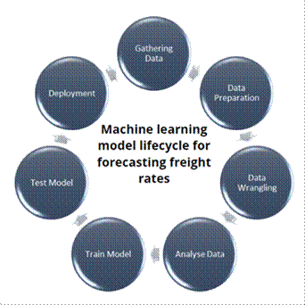
Fig. 2. Machine Learning Model Lifecycle

The dataset presents 3 types of variables: "object", "float64" and "int64". The variable type "int" is integer and "float" is floating point. The "object" variable is a value that represents a non-numeric value [51].

The distance category determines the number of kilometers in each country. The number of countries is limited to those through which the transports from the research sample arrived.

The relationship describes the initial loading location and the last unloading location. This is done using a postcode consisting of 2 letters and 5 numbers. For countries with a 4-digit code, the last one is completed as 0 to standardize the notation.

Date describes the date and time of the first loading and last unloading. The feature is represented as a range from to. The cargo category contains all the features related to the specifications of the goods. The organizational category describes other features.

Tab. 1

Key data about the dataset

Feature Category	Feature Name	Dtype	Completeness of Data
Distance	AT_KM	float64	100.00%
Distance	BE_KM	float64	100.00%
Distance	CZ_KM	float64	100.00%
Distance	DE_KM	float64	100.00%
Distance	DK_KM	float64	100.00%
Distance	EE_KM	float64	100.00%
Distance	ES_KM	float64	100.00%
Distance	FI_KM	float64	100.00%
Distance	HR_KM	float64	100.00%
Distance	FR_KM	float64	100.00%
Distance	HU_KM	float64	100.00%
Distance	IT_KM	float64	100.00%
Distance	LT_KM	float64	100.00%
Distance	LV_KM	float64	100.00%
Distance	NL_KM	float64	100.00%
Distance	PL_KM	float64	100.00%
Distance	RO_KM	float64	100.00%
Distance	SE_KM	float64	100.00%
Distance	SI_KM	float64	100.00%
Distance	SK_KM	float64	100.00%
Relation	COD_LP	object	100.00%
Relation	COD_DP	object	100.00%
Date	START_LOAD_DATA	object	100.00%
Date	START_LOAD_TIME	object	4.26%
Date	END_LOAD_DATA	object	100.00%
Date	END_LOAD_TIME	object	4.04%
Date	START_DELIVERY_DATA	object	100.00%
Date	START_DELIVERY_TIME	object	3.13%
Date	END_DELIVERY_DATA	object	100.00%
Date	END_DELIVERY_TIME	object	3.31%
Date	TIME_OF_ENTRY	object	89.63%
Cargo	GOODS_TYPE	object	93.81%
Cargo	BODY_TYPE	object	99.85%
Cargo	VEHICLE_TYPE	object	100.00%
Cargo	LOAD_UNLOAD_METHOD	object	99.96%
Cargo	REQUIREMENTS	object	0.07%
Cargo	EPALE	int64	100.00%
Cargo	LDM	float64	100.00%
Cargo	TONS	float64	100.00%
Cargo	M3	float64	100.00%
Cargo	HEIGHT	float64	0.11%
Cargo	WIDTH	float64	100.00%
Cargo	CARGO_VALUE_EURO	float64	0.07%
Cargo	TEMP_MIN	float64	0.73%
Cargo	TEMP_MAX	float64	0.73%
Organizational	OTHER_COSTS	float64	100.00%
Organizational	QTY_LOADS	float64	100.00%
Organizational	QTY_DELIVERIES	float64	100.00%
Organizational	PAYMENT TERM	float64	95.34%
Organizational	DOCUMENTS_BY	object	90.47%
Organizational	CUSTOMS	int64	100.00%

Tab. 2 presents basic statistical data for raw numerical features. Based on the distance features, we created a new one called "KM". It is simply the sum of kilometers across all countries. Before analyzing the "KM" feature, it is worth paying attention to the fact that a driver can work 13 hours between daily rests and extend this time to 15 hours 3 times a week. The driving time is 9 hours and can be extended to 10 hours twice a week [52]. Working time, which is not driving time, most often includes other activities related to loading and unloading goods. This should be taken into account when analyzing the data. As the statistics in the table show. The study sample represents a large set of short transports. Due to the limited possibilities of using working time for driving, such transports may be more expensive per kilometer. It can be assumed that a driver can cover 600 - 700 km a day if other activities do not affect his driving time. The median is 382.4, which shows that more than half of the transports are short. It can be concluded that the 25% group constitutes long transports (q3 = 710).

The "EPALE" feature is the number of pallets that the vehicle needs to exchange at the loading site. It is an abbreviation of "E Pallet Exchange". Statistical analysis clearly shows that most transports do not require such an exchange.

The "LDM" feature comes from the abbreviation "loading meters". The loading meters on the trailer are 2.4 meters wide. The length of the cargo space in a set consisting of a tractor unit and a semi-trailer is 13.6. After statistical analysis, it is concluded that the data relates entirely to full truckload transport. The situation is similar in the case of width, volume and weight.

Other costs concern a small group of shipments.

Transports most often have 1 loading and 1 unloading point and rarely require customs clearance.

Tab. 2

Statistical analysis of raw numerical input data

Feature			V	q2	Min.	Max.	q1	q3	q	Vq
KM	438.21	412.81	94.20	382.4	1	2439.5	53.6	710.0	328.2	85.83
EPALE	0.06	1.37	2194.02	0	0	34	0	0	0	-
LDM	13.6	0.01	0.06	13.6	13.2	13.6	13.6	13.6	0	0
TONS	24.57	2.15	8.73	25	1.52	25.7	25	25	0	0
M3	84.70	0.72	0.84	84.68	84.68	120	84.68	84.68	0	0
WIDTH	2.4	0	0	2.4	2.4	2.4	2.4	2.4	0	0
OTHER_COSTS	-3.95	45.96	-1164.81	0	-898.71	0	0	0	0	-
QTY_LOADS	1.01	0.10	10.35	1	1	4	1	1	0	0
QTY_DELIVERIES	1.02	0.19	18.59	1	1	6	1	1	0	0
CUSTOMS	0	0.04	2619.64	0	0	1	0	0	0	-

The next step is to examine the correlations between the features.

Fig. 3 presents a correlation matrix between features. We used Pearson's correlation for this. It should be remembered that, in principle, not everything that correlates with each other is dependent. The data concerns all data without division by qualitative variables. We would like to draw attention to the very high correlation between distance and price, equal to 0.92. This relationship is obviously expected. Before the analysis, the question was not whether there was a correlation, but how strong it was. The second important relationship resulting from the correlation matrix is the inverse proportionality of the price per kilometer to the distance. This confirms the above-mentioned issue that short transports are more expensive per kilometer than longer ones. There was no correlation between the price per kilometer and the number of loading and unloading operations, customs clearance and the number of pallets to be replaced. The fact that these dependencies do not result from this matrix does not mean that such dependencies do not exist.

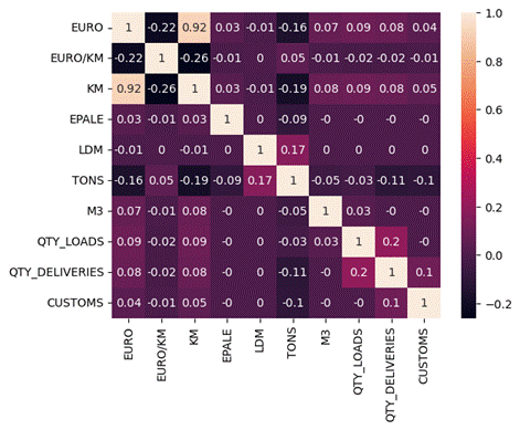
Fig. 3. Correlation Matrix

We did a more thorough analysis of the distance variable. We made a histogram of the distribution of the distance variable "KM" shown in

Fig. 4. Bins are placed every 100 kilometers. Signatures on the X axis every 500 kilometers. The average is marked with a red line. The median is marked with a green line. The statement made based on the statistical data from the table is confirmed. Short transports predominate. Additionally, an irregular distribution of the variable is observed.

The sum of kilometers from the entire research sample is over 1.2 million kilometers.

Fig. 5. Bar chart of kilometers by country shows the distribution of this by country of occurrence. More than half of the kilometers from the research sample are in Poland. Germany accounts for more than a quarter. This means that less than a quarter goes to other countries.

Tab. 3 shows the processing of all distance features. All raw data remain unchanged in the model. One new feature is the sum of all the others, denoted KM.

For the purposes of this work, relations are understood as the unique combination of loading and unloading countries. Fig. 6 shows a heatmap of average prices per kilometer in the relationship. The values shown in the chart are prices with additional costs subtracted. We calculated them using the following formula:

(1)

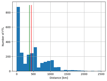
Fig. 4. Histogram of the distribution of the distance variable

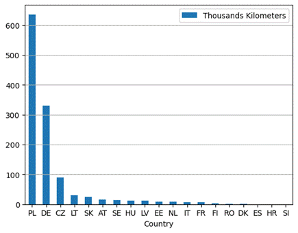
Fig. 5. Bar chart of kilometers by country

The analyzed research sample does not present transports in every relation. Full data only apply to transports from and to Poland. The highest price is presented in the domestic report in Poland. This is related to the large group of short transports on this route.

Tab. 3

Processing distance feature data

Raw Feature	Processed Feature
AT_KM	AT_KM
BE_KM	BE_KM
CZ_KM	CZ_KM
DE_KM	DE_KM
DK_KM	DK_KM
EE_KM	EE_KM
ES_KM	ES_KM
FI_KM	FI_KM
HR_KM	HR_KM
FR_KM	FR_KM
HU_KM	HU_KM
IT_KM	IT_KM
LT_KM	LT_KM
LV_KM	LV_KM
NL_KM	NL_KM
PL_KM	PL_KM
RO_KM	RO_KM
SE_KM	SE_KM
SI_KM	SI_KM
SK_KM	SK_KM
	KM

The analyzed research sample does not present transports in every relation. Full data only apply to transports from and to Poland. The highest price is presented in the domestic report in Poland. This is related to the large group of short transports on this route.

Tab. 4 shows the process of processing relation features. The raw data only contains the codes of the initial loading location and the last unloading location. On their basis, the country of loading and unloading are determined. On their basis, another feature called "RELATION" is created. This is a unique combination of loading and unloading country. For each unique value, We calculated: mean, median and standard deviation. Based on this, we created new features. The same way for "COUNTRY_LOAD_PLACE", "COUNTRY_DELIVERY_ PLACE" and "RELATION".

Fig. 7 shows the variable year distribution histogram. The number of transports from 2018 and 2019 is very small. The largest number of transports in the set are from 2020-2022.

Tab. 5 shows the process of creating date features. There are 4 features for the date and 5 features for the time. The time data is entered unchanged. The date data needs to be processed. We processed the date obtaining the following information: year, month, week of the year, day of the year, day of the week and day of the month.

We analyzed the seasonality in international transport. The results are shown in the Fig. 8. The minimum price is in January and the maximum in May.

An upward trend is visible between January and May. The exception to this trend is April. The price in April is lower than in March. However, the upward trend between March and May is maintained.

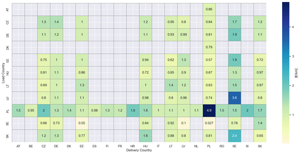
Fig. 6. Heatmap of average rates per kilometer in the relation

Tab. 4

Processing of relation data

Raw Feature	Processed Feature
COD_LP	COUNTRY_LOAD_PLACE_FACTORIZED
	COUNTRY_LOAD_PLACE_MEAN
	COUNTRY_LOAD_PLACE_MEDIAN
	COUNTRY_LOAD_PLACE_STD
COD_DP	COUNTRY_DELIVERY_PLACE_FACTORIZED
	COUNTRY_DELIVERY _PLACE_MEAN
	COUNTRY_DELIVERY _PLACE_MEDIAN
	COUNTRY_DELIVERY _PLACE_STD
	RELATION_PLACE_FACTORIZED
	RELATION_DELIVERY _PLACE_MEAN
	RELATION_DELIVERY _PLACE_MEDIAN
	RELATION_DELIVERY _PLACE_STD

Similarly, a downward trend is visible between May and January. The exception to this trend is September, when the price is lower than in October. However, the downward trend between August and October is maintained.

Tab. 6 shows the cargo data processing. The creation of features here should be divided into 2 methods. The first involves calculating: mean, median, standard deviation and assigning a category to each variable through factorization. This applies to the following features: goods type, body type, vehicle type, load and unload method, requirements.

The second one is to use the numerical feature as it is, this applies to the following features: euro pallets exchange, loading meters, tons, m³, height, width.

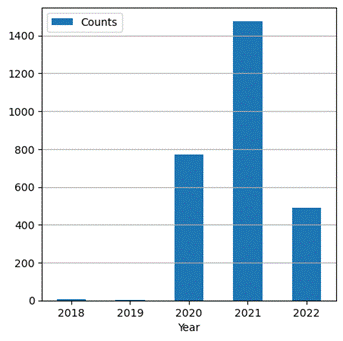
Fig. 7. Histogram of the year variable

Tab. 5

Date data processing

Raw Feature	Processed Feature
START_LOAD_DATA	START_LOAD_DATA_DAY
	START_LOAD_DATA_WEEKDAY
	START_LOAD_DATA_DAY_OF_YEAR
	START_LOAD_DATA_WEEK
	START_LOAD_DATA_MONTH
	START_LOAD_DATA_YEAR
START_LOAD_TIME	START_LOAD_TIME
END_LOAD_DATA	END_LOAD_DATA _DAY
	END_LOAD_DATA _WEEKDAY
	END_LOAD_DATA _DAY_OF_YEAR
	END_LOAD_DATA _WEEK
	END_LOAD_DATA _MONTH
	END_LOAD_DATA _YEAR
END_LOAD_TIME	END_LOAD_TIME
START_DELIVERY_DATA	START_DELIVERY_DATA _DAY
	START_DELIVERY _DATA _WEEKDAY
	START_DELIVERY _DATA _DAY_OF_YEAR
	START_DELIVERY _DATA _WEEK
	START_DELIVERY _DATA _MONTH
	START_DELIVERY _DATA _YEAR
START_DELIVERY_TIME	START_DELIVERY_TIME
END_DELIVERY_DATA	END_DELIVERY_DATA _DAY
	END_DELIVERY_DATA _WEEKDAY
	END_DELIVERY_DATA _DAY_OF_YEAR
	END_DELIVERY_DATA _WEEK
	END_DELIVERY_DATA _MONTH
	END_DELIVERY_DATA _YEAR
END_DELIVERY_TIME	END_DELIVERY_TIME
TIME_OF_ENTRY	TIME_OF_ENTRY

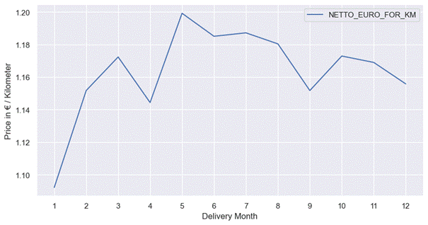
Fig. 8. Price depends on the month

Tab. 6

Cargo data processing

Raw Feature	Processed Feature
GOODS_TYPE	GOODS_TYPE_FACTORIZED
	GOODS_TYPE_MEAN
	GOODS_TYPE_MEDIAN
	GOODS_TYPE_STD
BODY_TYPE	BODY_TYPE _FACTORIZED
	BODY_TYPE _MEAN
	BODY_TYPE _MEDIAN
	BODY_TYPE _STD
VEHICLE_TYPE	VEHICLE_TYPE _FACTORIZED
	VEHICLE_TYPE _MEAN
	VEHICLE_TYPE _MEDIAN
	VEHICLE_TYPE _STD
LOAD_UNLOAD_METHOD	LOAD_UNLOAD_METHOD _FACTORIZED
	LOAD_UNLOAD_METHOD _MEAN
	LOAD_UNLOAD_METHOD _MEDIAN
	LOAD_UNLOAD_METHOD _STD
REQUIREMENTS	REQUIREMENTS_FACTORIZED
	REQUIREMENTS_MEAN
	REQUIREMENTS_MEDIAN
	REQUIREMENTS_STD
EPALE	EPALE
LDM	LDM
TONS	TONS
M3	M3
HEIGHT	HEIGHT
WIDTH	WIDTH

Fig. 9 shows body type variable distribution. The data is not diverse. The dominant body type is the standard type. All types whose number was less than 10 were marked as other.

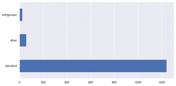
Fig. 9. Distribution of the body type variable

Tab. 7 shows the median rate per km of route by body type. The most expensive is the refrigerator. This is related to increased vehicle operating costs. This type of vehicle has refrigeration equipment that consumes fuel and generates costs.

The analysis of the distribution of the commodity type variable is presented in Fig. 10. The item type that occurred once was replaced with the "other" value. The dominant share of steel in the test sample is clearly visible.

Fig. 11 shows the distribution of the loading/unloading type variable. The most common method is a combination of all possible methods.

Tab. 8 shows the median price per kilometer according to the loading/unloading method required by the client.

We introduced the features prepared according to the description in the previous chapter into the models. We selected 5 different machine learning models for comparison. They were compared with each other according to the MAPE (Mean Absolute Percentage Error) metric. The results are shown in Fig. 12.

In the next step, we check what features were most important for the best XGBRegressor model. We use the eli5 library for this purpose. Fig. 13 shows the most important features for the model along with its weight. We will look at the importance of features from the perspective of the categorization described in section 3. The most important is distance (0.28 KM, 0.05 SE_KM).

Tab. 7

Median rate per km of route by body type

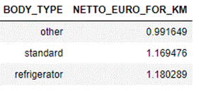
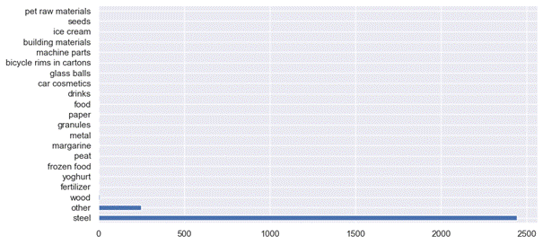
Fig. 10. Distribution of the goods type variable

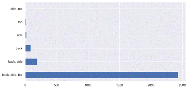
Fig. 11. Distribution of the load/unload method variable

Tab. 8

Median rate per km of route by load/unload method

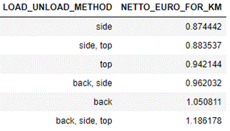
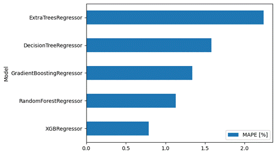
Fig. 12. Comparison of MAPE models

The second most important category is relationship (0.16 RELATION_MEDIAN, 0.12 COUNTRY_DELIVERY_MEAN, 0.08 COUNTRY_DELIVERY_PLACE, 0.07 START_DELIVERY_DATA_YEAR, 0.06 RELATION_MEAN, 0.02 COUNTRY_DELIVERY_MEDIAN, 0.02 RELATION, 0.01 COUNTRY_LOAD_PLACE, 0.01 LOAD_COUNTRY_MEAN, 0.01 COUNTRY_DELIVERY_STD).

The most important features also include those related to the cargo (0.02 GOODS_TYPE_MEDIAN, 0.01 M3, 0.01 LOAD_UNLOAD_METHOD_MEAN).

The least important categories are organizational features (0.02 OTHER_COSTS) and date features (0.01 END_DELIVERY_DATA_YEAR).

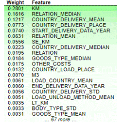
Fig. 13. Top 20 most important model features

4. DISCUSSION

The test results of the machine learning model for forecasting freight rates revealed many dependencies that can be observed in the market of European road transport services. Nowakowska-Grunt and Strzelczyk [53] deduced that road transport has the largest share in the transport of goods in the European Union. Generally, in 2021, total EU road freight transport accounted for around 1,921 billion ton-kilometers (tkm), 6.5% more than in 2020. In 2021 the overall national road freight transport in the EU accounted for 1 178.3 billion ton-kilometers, which is 6.3 % more than in 2020. In general, international road freight transport in the EU ac-counted for around 743.2 billion ton-kilometers, which is 6.9 % more than in 2020 [54]. Both the statistics and the results of the model indicate a greater share of short-distance transport in road transport carried out within the EU. The transport of goods by road is most often carried out within the area of one country or, due to the high density of European countries, it is associated with the exchange of goods be-tween neighboring countries. Statistical data related to transport performance by distance class are different from the results of model research. Road freight rate data are sensitive and hard to access. Differences in results are due to the relatively small sample of data compared to Eurostat data. However, the use of the methodology proposed in this study and a larger data set will allow one to create better models. In 2021, most goods were transported within the EU and for most EU countries over distances be-tween 300 and 999 km (40.8%). However, several countries showed a different pattern of transport performance depending on the distance class. Particularly for some islands and countries (Ireland, Cyprus, the Netherlands, and Austria) where the domestic market plays an important role, the share of short-distance road freight transport (less than 150 km) was higher. For example, in Cyprus, more than 90% of transport is less than 150 km. On the other hand, countries, where international road transport plays a key role, have a higher share of long-distance transport (above 1,000 km). For example, transport over this distance accounts for 50.8% of the number of ton-kilometers in Lithuania, 48.8% in Portugal, 46.2% in Bulgaria and 40.0% in Latvia [55]. Differences resulting from the model results and statistics of the model may be related to the fact that only full truck loads were considered in the data set.

As suggested by Inkinen and Hämäläinen [56], long-distance journeys are typical for hinterland transportation, while short distances are dominant in intra-urban transportation, as they are used for last mile customer door-to-door deliveries. Zgonce et al. [57] examined the hypothesis that distance is one of the most important factors that influence the choice of mode in freight transport. The results showed that intermodal transport can provide a competitive alternative to unimodal road transport for long distances. That is why the distance feature in the model can be important information for researchers dealing with modal shifts. For example, Boer et al. [58] analyze various studies to estimate the potential of shifting from road and air transport to rail, as well as the volume of goods physically suitable for the change. According to the results, the potential for a modal shift from the road to rail is 100% for distances greater than 500 km, 40% for 150–500 km and only 5% for 50-150 km.

The weekly seasonality of the freight rates that were observed in the test results was correlated with different EU regions. This is due to the unsustainable development of countries in terms of the price of human labor. As Kot [59] presents in his research, employment costs are the second most important factor after full costs for most transport companies. Workers from lower-wage countries want to spend their week's rest at their place of residence. This is because, as Luekewille et al. [60] underline, labor costs are included in several country-specific circumstances, in addition to the level of technological advancement, the size distribution, etc., which have an impact on the differentiation of the functioning of the transport systems. Poliak et al. [61] deal with the issue of insufficient harmonization of social conditions concerning the remuneration of drivers involved in road transport. This causes an unbalanced demand-supply situation. If in the future the development of countries is more sustainable, the impact of weekly seasonality on the price of the service will decrease.

According to the generalized transport cost (GTC) concept, the maps shown by Persyn et al. [62] reveal that the regions with a less developed road network, such as in Eastern Europe show the largest reduction in internal transport costs. Considering distance and time dimensions in the GTC, the paper allowed one to disentangle core-periphery structures of the EU regions due to transport costs. According to the developed freight rate model test results, the highest prices for road carriage are paid for destination: Slovakia – Sweden (about 2.35 €/km) and Sweden-Slovakia (about 2.31 €/km). This is very important information for fleet managers and owners of transport companies regarding the selection of transport orders in these relations. In turn, in the relations of transport corridors Estonia-Poland (about 0.57 €/km) and Sweden-Poland (about 0.53 €/km), the earning potential is the lowest, although it is not only affected by the margin but also by other cost components, such as fuel or vignettes. This is confirmed by the research of Poliak et al. [63], whose analysis shows that the direction of transportation is a significant offer factor and, therefore, it is appropriate to include this factor in price creation. A comparison of the results of the application of the route utilization coefficient for specific countries shows the differences in transport prices. Based on the studies, the differences are particularly visible for those countries where the level of transport supply is very low (e.g., France and Luxembourg). Furthermore, Liachoviius and Skrickij [64] as well as Konen et al. [65] indicate that the tax burden and charges in road freight transport are significantly different in EU countries. Hajek et al. [66] examined how the particular impact of transport tax revenues on GHG emissions varied between countries. Therefore, it is very important to monitor the sustainable development and progress of the sector. In their research, Siksnelyte-Butkiene and Streimikiene [67] seek to develop a framework for the sustainability assessment of road transport and assess the achievements in EU countries.

The decision on the relationship between freight rate and the type of vehicle body may be important in the case of investment plans implemented in transport companies. The test results of the model presented refrigerated trucks to be the most profitable. However, as shown by Amaruchkul et al. [68], the determination of the cycle time of each product, the temperature of each zone in each truck, and the allocation plan that specifies how many units of each product would be delivered in each zone in each truck is a complex problem. That is why transportation companies prefer to use more universal body types. The largest number of trucks is in Poland, followed by Italy and Germany, and as Kubáová et al. [69] investigated, the European truck market is dominated by manufacturers. Daimler Trucks, MAN Truck and Bus, Volvo Trucks, Scania, DAF, and Iveco. This is the reason why the aspect of sustainable transport is probably a more important decision-making factor than vehicle unit profitability. According to ACEA reports [70], there are currently more than 6 million trucks in use in the EU and the average age of European trucks is 12 years and 98.3% of all heavy and medium trucks (more than 3.5 tons) on Europe’s roads today run on diesel.

5. CONCLUSIONS

The paper concerned the problem of the construction of freight rates and components in road transport. Forecasting freight prices is a complex task that involves considering various factors and variables that can affect pricing dynamics in the sustainable transportation industry and business. Therefore, scientists experiment with different techniques and evaluate their performance using appropriate metrics to find the best solution for a specific prediction task. The theoretical analysis of previous publications revealed research especially visible in the field of road transportation freight rate forecasting. However, through a literature review, great opportunities offered by artificial intelligence techniques, including machine learning, which can be used to predict transport prices have also been noticed.

For this reason, the road freight rate forecasting model based on the machine learning lifecycle procedure was proposed as a supporting tool in sustainable road transport decision-making. The model is based on the most important features of freight rates: distance, relation, vehicle type, body type, or other characteristics which can be applied to the method depending on own needs. The results of the model test were carried out based on 2748 datasets of 2,688 full truck load transport services offers (FTL) collected in the freight exchange market during the years 2018-2022. The analysis revealed interesting mechanisms of freight rate creation in the European market. The analyzed results also indicated the sensitivity of the model to the size of the database used in the machine learning method.

The analysis allowed us to conclude that machine learning models can be effective in forecasting freight prices in the context of sustainable transport due to their ability to capture complex patterns and relationships in large datasets. The application of the described method supports stable, sustainable, and inclusive economic growth. It allows smaller businesses in the poorest areas to take advantage of advanced technology, leveling the playing field. The use of the above methodology allows you to delegate time-consuming tasks that require a lot of computing power to the model. At the same time, human resources for tasks that require natural intelligence, such as building relationships with contractors. The use of the model for decision-making in the management of transport processes, which on a global scale allows you to make better decisions that can reduce empty runs.

The current situation is the requirement of customers for the appropriate exhaust gas emission standard. We assume that in the future there may be similar requirements for alternative energy sources such as electricity and hydrogen. By collecting enough data on transport using alternative energy sources, we can train a model that takes this into account. The methodology presented in this article can be used to process energy source data. The use of such an approach will make it possible to assess the costs of using ecological energy sources on individual routes.

References

1. Behar Alberto, Venables Anthony. 2011. „Transport costs and international trade. A handbook of transport economics. In A Handbook of Transport Economics , edited by André de Palma, Robin Lindsey, Emile Quinet, and Roger Vickerman, 97. ISBN: 9781847202031.

2. UNCTAD. 2022. „Review of maritime transport” In: Proceedings of the United Nation Conference on Trade and Development. Genewa

3. Placek Martin. „Road freight transport revenue worldwide 2019-2022”. Available at: https://www.statista.com/statistics/1288518/road-freight-transport-revenue-worldwide.

4. Eurostat. „International trade in goods by mode of transport”. Available at: https://ec.europa.eu/eurostat/statistics-explained/index.php?title=International_trade_in_goods_by_mode_of_transport.

5. Ti-insight. „European Road Freight Transport 2023”. 2023. Report. Bath, UK.

6. Schnepf Randy. 2006. „Price determination in agricultural commodity markets: a primer”. Congressional Research Service, Library of Congress. Available at: http://research.policyarchive.org/2678.pdf.

7. Volpe Richard, Roeger Edward, Leibtag Ephraim. 2013. How transportation costs affect fresh fruit and vegetable prices. Washington: Department of Agriculture, Economic Research Service.

8. Melas Konstantinos, Michail Nektarios. 2021. „The relationship between commodity prices and freight rates in the dry bulk shipping segment: A threshold regression approach”. Maritime Transport Research. ISSN: 2666-822X. DOI: https://doi.org/10.1016/j.martra.2021.100025.

9. De Bok Michiel, Bart Wesseling, Jan Kiel, Onno Miete, Jan Francke. „A sensitivity analysis of freight transport forecasts for The Netherlands”. International Journal of Transport Economics. 45(4): 571-587. DOI: https://doi.org/10.19272/201806704003.

10. Saeed, Naima, Su Nguyen, Kevin Cullinane, Victor Gekara, and Prem Chhetri. „Forecasting Container Freight Rates Using the Prophet Forecasting Method”. Transport Policy 133(2023): 86-107. DOI: https://doi.org/10.1016/j.tranpol.2023.01.012.

11. Nielsen Peter, Liping Jiang, Niels Gorm, Malý Rytter, Gang Chen. 2014. „An Investigation of Forecast Horizon and Observation Fit’s Influence on an Econometric Rate Forecast Model in the Liner Shipping Industry”. Maritime Policy & Management 41(7): 667-82. DOI: https://doi.org/10.1080/03088839.2014.960499.

12. Chen, Yanhui, Bin Liu, Tianzi Wang. 2021. „Analysing and Forecasting China Containerized Freight Index with a Hybrid Decomposition-Ensemble Method Based on EMD, Grey Wave and ARMA”. Grey Systems: Theory and Application 11(3): 358-71. ISSN: 2043-9377. DOI: https://doi.org/10.1108/GS-05-2020-0069.

13. Jeon, Jun-Woo, Okan Duru, Ziaul Haque Munim, Naima Saeed. 2021. „System Dynamics in the Predictive Analytics of Container Freight Rates”. Transportation Science 55(4): 946-67. ISSN: 0041-1655. DOI: https://doi.org/10.1287/trsc.2021.1046.

14. Munim, Ziaul Haque, Hans-Joachim Schramm. 2017. „Forecasting Container Shipping Freight Rates for the Far East – Northern Europe Trade Lane”. Maritime Economics & Logistics 19(1): 106-25. ISSN: 1479-2931. DOI: https://doi.org/10.1057/s41278-016-0051-7.

15. Schramm, Hans-Joachim, Ziaul Haque Munim. 2021. „Container Freight Rate Forecasting with Improved Accuracy by Integrating Soft Facts from Practitioners”. Research in Transportation Business & Management 41 (December): 100662. ISSN: 2210-5395. DOI: https://doi.org/10.1016/j.rtbm.2021.100662.

16. Slack, Brian, Elisabeth Gouvernal. 2011. „Container Freight Rates and the Role of Surcharges”. Journal of Transport Geography 19 (6): 1482-89. ISSN: 0966-6923. DOI: https://doi.org/10.1016/j.jtrangeo.2011.09.003.

17. Batchelor, Roy, Amir Alizadeh, Ilias Visvikis. 2007. „Forecasting Spot and Forward Prices in the International Freight Market”. International Journal of Forecasting 23(1): 101-14. ISSN: 0169-2070. DOI: https://doi.org/10.1016/j.ijforecast.2006.07.004.

18. Chen, Shun, Hilde Meersman, Eddy Van De Voorde. 2012. „Forecasting Spot Rates at Main Routes in the Dry Bulk Market”. Maritime Economics & Logistics 14(4): 498-537. ISSN: 1479-2931. DOI: https://doi.org/10.1057/mel.2012.18.

19. Li, Kevin X., Yi Xiao, Shu-Ling Chen, Wei Zhang, Yuquan Du, Wenming Shi. 2018. „Dynamics and Interdependencies among Different Shipping Freight Markets”. Maritime Policy & Management 45(7): 837-49. https://doi.org/10.1080/03088839.2018.1488187.

20. Dikos George, Henry S. Marcus, Martsin Panagiotis Papadatos, Vassilis Papakonstantinou. 2006. „Niver Lines: A System-Dynamics Approach to Tanker Freight Modeling”. Interfaces 36(4): 326-41. https://doi.org/10.1287/inte.1060.0218.

21. Kabir Abdulmajeed, Monsuru Adeleke, Labode Popoola. 2020. „Online forecasting of COVID-19 cases in Nigeria using limited data”. Data in Brief 30: 105683. ISSN: 2352-3409. DOI: https://doi.org/10.1016/j.dib.2020.105683.

22. Kasimati Evangelia, Nikolaos Veraros. 2018. „Accuracy of Forward Freight Agreements in Forecasting Future Freight Rates”. Applied Economics 50(7): 743-56. ISSN: 0003-6846. DOI: https://doi.org/10.1080/00036846.2017.1340573.

23. Munim Ziaul Haque. 2022. „State-Space TBATS Model for Container Freight Rate Forecasting with Improved Accuracy”. Maritime Transport Research 3: 100057. ISSN: 2666-822X. DOI: https://doi.org/10.1016/j.martra.2022.100057.

24. Duru Okan, Emrah Gulay, Korkut Bekiroglu. 2023. „Predictability of the Physical Shipping Market by Freight Derivatives”. IEEE Transactions on Engineering Management 70(1): 267-79. ISSN: 0018-9391. DOI: https://doi.org/10.1109/TEM.2020.3046930.

25. Lam Jasmine Siu Lee, Qingyao Li, Shuyi Pu. 2021. „Volatility and Uncertainty in Container Shipping Market“. In: New Maritime Business, edited by Byoung-Wook Ko and Dong-Wook Song, 10: 11-32. WMU Studies in Maritime Affairs. Cham: Springer International Publishing. ISBN: 978-3-030-78956-5 978-3-030-78957-2.

26. Choudhary, Ankur, Santosh Kumar, Manish Sharma, K.P. Sharma. 2022. „A Framework for Data Prediction and Forecasting in WSN with Auto ARIMA”. Wireless Personal Communications 123(3): 2245-59. ISNN: 0929-6212. DOI: https://doi.org/10.1007/s11277-021-09237-x.

27. Al-Qazzaz Redha Ali, Suhad Yousif. 2022. ”High Performance Time Series Models Using Auto Autoregressive Integrated Moving Average”. Indonesian Journal of Electrical Engineering and Computer Science 27(1): 422. ISSN: 2502-4760. DOI: https://doi.org/10.11591/ijeecs.v27.i1.pp422-430.

28. Nguyen Huy Vuong, M. Asif Naeem, Nuttanan Wichitaksorn, Russel Pears. 2019. „A Smart System for Short-Term Price Prediction Using Time Series Models”. Computers & Electrical Engineering 76(June): 339-52. ISSN: 0045-7906. DOI: https://doi.org/10.1016/j.compeleceng.2019.04.013.

29. Kumar Dubey Ashutosh, Abhishek Kumar, Vicente García-Díaz, Arpit Kumar Sharma, Kishan Kanhaiya. 2021. ‚Study and Analysis of SARIMA and LSTM in Forecasting Time Series Data”. Sustainable Energy Technologies and Assessments 47(October): 101474. ISSN: 2213-1388 https://doi.org/10.1016/j.seta.2021.101474.

30. Makridakis Spyros, Evangelos Spiliotis, Vassilios Assimakopoulos. 2020. „The M4 Competition: 100,000 Time Series and 61 Forecasting Methods”. International Journal of Forecasting 36(1): 54-74. ISSN: 0169-2070. DOI: https://doi.org/10.1016/j.ijforecast.2019.04.014.

31. Mazanec Jaroslav, Veronika Harantová, Vladimíra Štefancová, Hana Brůhová Foltýnová. 2023. „Estimating Mode of Transport in Daily Mobility during the COVID-19 Pandemic Using a Multinomial Logistic Regression Model”. International Journal of Environmental Research and Public Health 20(5): 4600. ISSN: 1660-4601. DOI: https://doi.org/10.3390/ijerph20054600.

32. Al Hasan Mohammad, Li Xiong. 2022. „Do simpler statistical methods perform better in multivariate long sequence time-series forecasting? ”. In: Proceedings of the 31st ACM International Conference on Information & Knowledge Management. Atlanta GA USA: ACM.

33. Hyndman, Rob J., Yeasmin Khandakar. 2008. „Automatic Time Series Forecasting: The Forecast Package for R”. Journal of Statistical Software 27(3). ISSN: 1548-7660. DOI: https://doi.org/10.18637/jss.v027.i03.

34. Navratil Miroslav, Andrea Kolkova. 2019. „Decomposition and Forecasting Time Series in the Business Economy Using Prophet Forecasting Model”. Central European Business Review 8(4): 26-39. ISSN: 18054854. DOI: https://doi.org/10.18267/j.cebr.221.

35. Papacharalampous Georgia A., Hristos Tyralis. 2018. „Evaluation of Random Forests and Prophet for Daily Streamflow Forecasting”. Advances in Geosciences 45(August): 201-8. ISSN: 1680-7359. DOI: https://doi.org/10.5194/adgeo-45-201-2018.

36. Chuwang Dung David, Weiya Chen. 2022. „Forecasting Daily and Weekly Passenger Demand for Urban Rail Transit Stations Based on a Time Series Model Approach”. Forecasting 4(4): 904-24. ISSN: 2571-9394. DOI: https://doi.org/10.3390/forecast4040049.

37. Widodo Agus, Indra Budi, Belawati Widjaja. 2016. „Automatic Lag Selection in Time Series Forecasting Using Multiple Kernel Learning”. International Journal of Machine Learning and Cybernetics 7(1): 95-110. ISSN: 1868-8071. DOI: https://doi.org/10.1007/s13042-015-0409-7.

38. Mrowczynska Bogna, Maria Ciesla, Aleksander Krol, Aleksander Sladkowski. 2017. „Application of Artificial Intelligence in Prediction of Road Freight Transportation”. PROMET – Traffic&Transportation 29(4): 363-70. ISSN: 1848-4069. DOI: https://doi.org/10.7307/ptt.v29i4.2227.

39. Züfle Marwin, Samuel Kounev. 2020. „A Framework for Time Series Preprocessing and History-Based Forecasting Method Recommendation”. In: Proceedings of the 2020 Federated Conference on Computer Science and Information Systems, edited by M. Ganzha, L. Maciaszek, M. Paprzycki, ACSIS: 141-44.

40. Martínez Francisco, María Pilar Frías, María Dolores Pérez, Antonio Jesús Rivera. 2019. „A Methodology for Applying K-Nearest Neighbor to Time Series Forecasting”. Artificial Intelligence Review 52(3): 2019-37. ISSN: 0269-2821. DOI: https://doi.org/10.1007/s10462-017-9593-z.

41. Bogachev Taras, Tamara Alekseychik, Anatoly Chuvenkov, Svetlana Batygova. 2021. „Comparative Assessment of the Regional Freight Transportation by Method of Fuzzy Linear Regression”. In: 14th International Conference on Theory and Application of Fuzzy Systems and Soft Computing – ICAFS-2020, edited by Rafik A. Aliev, Janusz Kacprzyk, Witold Pedrycz, Mo Jamshidi, Mustafa Babanli, Fahreddin M. Sadikoglu, 1306: 102-9. Advances in Intelligent Systems and Computing. Cham: Springer International Publishing. ISBN: 978-3-030-64057-6 978-3-030-64058-3.

42. Khan Ibraheem Abdulhafiz, Farookh Khadeer Hussain. 2022. „Regression Analysis Using Machine Learning Approaches for Predicting Container Shipping Rates”. In: Advanced Information Networking and Applications, edited by Leonard Barolli, Farookh Hussain, and Tomoya Enokido, 450: 269-80. Lecture Notes in Networks and Systems. Cham: Springer International Publishing. ISBN: 978-3-030-99586-7. DOI: https://doi.org/10.1007/978-3-030-99587-4_23.

43. Koyuncu Kaan, Leyla Tavacioğlu. 2021. „Forecasting Shanghai Containerized Freight Index by Using Time Series Models”. Marine Science and Technology Bulletin 10(4): 426-34. ISSN: 2147-9666. DOI: https://doi.org/10.33714/masteb.1024663.

44. Bashir Sara, Milan Zlatkovic. 2021. „Assessment of Queue Warning Application on Signalized Intersections for Connected Freight Vehicles”. Transportation Research Record: Journal of the Transportation Research Board 2675(10): 1211-21. DOI: https://doi.org/10.1177/03611981211015247.

45. Gladchenko E.A., O.N. Saprykin, AN. Tikhonov. 2019. „Optimization of urban freight transportation based on evolutionary modelling”. In: CEUR Workshop Proceedings 2019”: 95-103.

46. Kluyver Thomas, Ragan-Kelley Benjamin, Pérez Fernando, Granger Brian, Bussonnier Matthias, Frederic Jonathan, Kelley Kyle, Hamrick Jessica, Grout Jason, Corlay Sylvain, Ivanov Paul, Avila Damián, Abdalla Safia, Willing Carol. 2016. „Jupyter Notebooks – a publishing format for reproducible computational workflows”. In: 20th International Conference on Electronic Publishing”: 87-90.

47. McKinney Wes. 2010. „Data Structures for Statistical Computing in Python”. In: Proc. of the 9th Python in Science Conf. (SCIPY 2010): 56-61. Austin, Texas. DOI: https://doi.org/10.25080/Majora-92bf1922-00a.

48. Waskom Michael. 2021. „Seaborn: Statistical Data Visualization”. Journal of Open Source Software 6(60): 3021. DOI: https://doi.org/10.21105/joss.03021.

49. Hunter John D. 2007. „Matplotlib: A 2D Graphics Environment”. Computing in Science & Engineering 9(3): 90-95. DOI: https://doi.org/10.1109/MCSE.2007.55.

50. Pedregosa Fabian, Gaël Varoquaux, Alexandre Gramfort, Vincent Michel, Bertrand Thirion, Olivier Grisel, Mathieu Blondel, et al. 2012. „Scikit-Learn: Machine Learning in Python”. arXiv: 1201.0490. DOI: https://doi.org/10.48550/ARXIV.1201.0490.

51. Built-in Types. The Python Standard Library. Available at: https://docs.python.org/3/library/stdtypes.html.

52. Eur-Lex. Regulation (EC) No 561/2006 of the European Parliament and of the Council of 15 March 2006 on the harmonisation of certain social legislation relating to road transport. 2006. Available at: https://eur-lex.europa.eu/legal-content/EN/ALL/?uri=CELEX%3A32006R0561.

53. Nowakowska-Grunt Joanna, Monika Strzelczyk. 2019. „The Current Situation and the Directions of Changes in Road Freight Transport in the European Union”. Transportation Research Procedia 39: 350-59. ISSN: 2352-1465. DOI: https://doi.org/10.1016/j.trpro.2019.06.037.

54. Eurostat. Road freight transport performance by type of operation, 2017-2021. Available at: https://ec.europa.eu/eurostat/databrowser/product/page/ROAD_GO_TA_TOTT.

55. Eurostat. Road freight transport performance by distance class, 2021. Available at: https://ec.europa.eu/eurostat/databrowser/view/ROAD_GO_TA_DC/default/table?lang=en&category=road.road_go.road_go_tot.

56. Inkinen Tommi, Esa Hämäläinen. 2020. „Reviewing Truck Logistics: Solutions for Achieving Low Emission Road Freight Transport”. Sustainability 12(17): 6714. DOI: https://doi.org/10.3390/su12176714.

57. Zgonc Borut, Metka Tekavčič, Marko Jakšič. 2019. „The Impact of Distance on Mode Choice in Freight Transport”. European Transport Research Review 11(1): 10. ISSN: 1867-0717. DOI: https://doi.org/10.1186/s12544-019-0346-8.

58. den Boer Eelco, Essen Huib, Brouwer Femke, Pastori Enrico, Moizo Alessandra. 2011. Potential of modal shift to rail transport-Study on the projected effects on GHG emissions and transport volumes. CE Delft. Publication No. 11.4255.15.

59. Kot Sebastian. 2015. ”Cost Structure in Relation to the Size of Road Transport Enterprises”. PROMET - Traffic&Transportation 27(5): 387-94. ISSN: 1848-4069. DOI: https://doi.org/10.7307/ptt.v27i5.1687.

60. Lükewille Anke, Imrich Bertok, Markus Amann, Janusz Cofala, Frantisek Gyarfas, Chris Heyes, Niko Karvosenoja, Zbigniew Klimont, Wolfgang Schöpp. 2021. A Framework to Estimate the Potential and Costs for the Control of Fine Particulate Emissions in Europe. IIASA Interim Report. IIASA, Laxenburg, Austria: IR-01-023.

61. Poliak Miloš, Patricia Šimurková, Kelvin Cheu. 2019. „Wage Inequality Across The Road Transport Sector Within the Eu”. Transport Problems 14(2): 145-53. ISSN: 1896-0596. DOI: https://doi.org/10.20858/tp.2019.14.2.13.

62. Persyn, Damiaan, Jorge Díaz-Lanchas, Javier Barbero. 2022. „Estimating Road Transport Costs between and within European Union Regions”. Transport Policy 124 (August): 33-42. ISSN: 0967-070X. DOI: https://doi.org/10.1016/j.tranpol.2020.04.006.

63. Poliak Milos, Adela Poliakova, Lucie Svabova, Natalia Aleksandrovna Zhuravleva, Elvira Nica. 2021. „Competitiveness of Price in International Road Freight Transport”. Journal of Competitiveness 13(2): 83-98. ISSN: 1804-171X. DOI: https://doi.org/10.7441/joc.2021.02.05.

64. Liachovičius Edvardas, Viktor Skrickij. 2020. „The Challenges and Opportunities for Road Freight Transport“. In: TRANSBALTICA XI: Transportation Science and Technology, edited by Kasthurirangan Gopalakrishnan, Olegas Prentkovskis, Irina Jackiva, Raimundas Junevičius, 455-65. Lecture Notes in Intelligent Transportation and Infrastructure. Cham: Springer International Publishing.

65. Konečný Vladimír, Semanová Štefánia, Gnap Jozef, Stopka Ondrej. 2018. ”Taxes and Charges in Road Freight Transport – a Comparative Study of the Level of Taxes and Charges in the Slovak Republic and the Selected EU Countries”. Naše More 65(4): 208-12. ISBN: 978-3-030-38665-8. DOI: https://doi.org/10.17818/NM/2018/4SI.8.

66. Hájek Miroslav, Jarmila Zimmermannová, Karel Helman. 2021. „Environmental Efficiency of Economic Instruments in Tansport in EU Countries”. Transportation Research Part D: Transport and Environment 100 (November): 103054. ISSN: 1361-9209. DOI: https://doi.org/10.1016/j.trd.2021.103054.

67. Siksnelyte-Butkiene Indre, Dalia Streimikiene. 2022. „Sustainable Development of Road Transport in the EU: Multi-Criteria Analysis of Countries Achievements”. Energies 15(21): 8291. ISSN: 1996-1073. DOI: https://doi.org/10.3390/en15218291.

68. Amaruchkul Kannapha, Akkaranan Pongsathornwiwat, Purinut Bantadtiang. 2022. „Constrained Joint Replenishment Problem with Refrigerated Vehicles”. Engineering Journal 26(1): 75-91. ISSN: 01258281. DOI: https://doi.org/10.4186/ej.2022.26.1.75.

69. Kubáňová Jaroslava, Iveta Kubasáková, Dočkalik. 2021. „Analysis of the Vehicle Fleet in the EU with Regard to Emissions Standards”. Transportation Research Procedia 53: 180-87. DOI: https://doi.org/10.1016/j.trpro.2021.02.024.

70. ACEA. Zero-emission trucks require radical policy changes, says ACEA as new fleet data is released. Available at: https://www.acea.auto/press-release/zero-emission-trucks-require-radical-policy-changes-says-acea-as-new-fleet-data-is-released/

Received 17.06.2024; accepted in revised form 05.10.2024

Scientific Journal of Silesian University of Technology. Series Transport is licensed under a Creative Commons Attribution 4.0 International License

---

[1] Institute of Quality Science and Product Management, The Cracov University of Economics, Rakowicka 27 Street, 31-510 Cracow, Poland. Email: abudzyns@uek.krakow.pl.
ORCID: https://orcid.org/0000-0002-5803-6749

[2] Faculty of Transport and Aviation Engineering, The Silesian University of Technology, Krasińskiego 8 Street, 40-019 Katowice, Poland. Email: maria.ciesla@polsl.pl. ORCID: https://orcid.org/ 0000-0003-4566-6554