Article citation information:
Özinal
Avşar, Y., Avşar, E. Short-term traffic state
estimation using breakpoint flow calculation and machine learning methods. Scientific Journal of Silesian University of
Technology. Series Transport. 2022, 115,
121-134. ISSN: 0209-3324. DOI: https://doi.org/10.20858/sjsutst.2022.115.9.
Yağmur ÖZİNAL
AVŞAR[1],
Ercan AVŞAR[2]
SHORT-TERM TRAFFIC STATE ESTIMATION USING BREAKPOINT FLOW CALCULATION
AND MACHINE LEARNING METHODS
Summary. Estimation of
the state of road traffic conditions is gaining increasing attention in
recent intelligent transportation systems. Accurate and real-time estimation of
traffic condition changes is critical in the management and control of road
network systems. Thus, efforts are been made to predict short-term traffic
conditions based on measured traffic data such as speed, flow and density. In
this work, the state of the traffic is estimated through a three-step process.
First, both speed and flow predictions for 15-minute ahead are made for a
particular freeway segment. Four different regression models are used for the
prediction task, namely, multi-layer perceptron neural networks (MLPNN),
support vector regression (SVR), gradient boosted decision trees (GBDT), and
k-nearest neighbors (kNN). Next, the breakpoint (BP) flow is calculated using
the distribution of these predicted speed and flow values. In the final step,
these predictions are classified as belonging to a “stable state”
or “metastable state” by using the calculated BP as the threshold
between these states. According to the experimental results, the values for
MLPNN are the highest for speed (0.8564) and flow (0.9862) predictions. An
identical BP, 1050 pc/15min, is calculated for actual data as well as all
prediction methods.
Keywords: breakpoint,
machine learning, short-term traffic, prediction, speed-flow relationship
1. INTRODUCTION
Intelligent
transportation systems (ITS) are being equipped with smart sensing, computation
and communication technologies to increase the operational efficiency and
capacity of transportation systems [1-3]. Thus, it is possible to collect data
related to traffic parameters accurately, reliably and in real-time. In
particular, advanced traffic management systems (ATMS) and advanced traveler
information systems (ATIS) need accurate and reliable traffic information to
predict traffic characteristics for transport users to understand and estimate
future traffic conditions. Hence, accurate and real-time traffic prediction has
been defined as a very critical need for the operational efficiency of ITS [4].
Data-driven
management and control of transportation systems have become possible as a
result of recent advancements in technology and computer science. Prediction of
traffic parameters has been a popular research subject since the late 1970s.
Consequently, short-term traffic prediction, which refers to estimating the
traffic conditions up to 60 minutes ahead, has been an essential part of ITS.
Such predictions help optimization of transport systems such as real-time
traffic management, development of control strategies, delay, congestion, and
energy consumption reduction.
The main
variables that form the traffic flow theory are speed, flow and density. These
variables alone cannot provide sufficient information to explain the irregular
nature of the traffic. Thus, the situation of traffic has been explained using
fundamental diagrams such as speed-density, density-flow and speed-flow
diagrams. These diagrams were first established by Greenshields [5] and later
improved by other researchers. Now, they form the basis of traffic theories and
models, besides, they are important subjects of traffic measurements and
teaching basis in the area of transportation. Since 1965, in all editions of
the Highway Capacity Manual (HCM), inspecting speed-flow diagrams have
constituted the basis of design and analysis methodologies for basic freeway
segments and uninterrupted flow segments of multilane highways. Furthermore,
these diagrams are used as the basic methodology for empirical studies of
measured traffic data.
Speed-flow
diagrams are used to determine the capacity and level of service in
uninterrupted flow segments of highways and basic freeway segments.
Additionally, the relationship between these variables is useful in detecting
the phase transition of traffic flow. The transition from stable flow to
metastable flow occurs at the breakpoint (BP). It is especially the point
separating the constant-speed portion of the curve in the diagram from the rest
of it. Stable free flow prevails up to BP and after this point, metastable free
flow is dominated present up to the maximum capacity value. BP is the point
where the traffic flow situation starts to change; therefore, it is important
to detect this point to understand the transition between stable traffic flow
and change in vehicle speed.
In the
existing literature, several efforts have been made to address the prediction
of traffic speed, density or flow; however, most of these studies only focus on
the predictions of one of these parameters. However, predicting traffic speed
or flow alone cannot explain traffic conditions adequately. Therefore, it is
necessary to determine the BP of flow after which the traffic speed starts to
decrease. Thus, proper identification of BP from the predicted values is
important to predict the transition of flow from stable to metastable state in
the short term [6].
Relevant
studies involve numerous methods for short-term traffic predictions. Van Lint and Van Hinsbergen [7] classified
the approaches used in short-term traffic predictions into four categories:
naïve, parametric, nonparametric and hybrid. These include the use of
machine learning methods such as the k-nearest neighbors (kNN) [8], support
vector regression (SVR) [9] and
artificial neural networks (ANN) [10].
In this work,
the state of traffic flow is estimated using the flow level corresponding to
BP. The BP value was determined from the predicted flow and speed values. To
achieve this, 15-minute ahead predictions are performed using four different
regression models, namely, multi-layer perceptron neural networks (MLPNN), SVR,
gradient boosted decision trees (GBDT), and kNN. Next, speed-flow diagrams for
predictions of each of these methods are generated to calculate BP. Rate of
change in standard deviations of speed against flow predictions is calculated
to determine the BP. Finally, the state of traffic flow is estimated by
checking which side of the calculated BP the predictions fall on. The main
contributions of this paper are (i) both speed and flow predictions are made
for a particular freeway segment, (ii) these predictions are analyzed together
to calculate BP, and (iii) traffic flow state is estimated using the
predictions and the calculated BP.
2.
BACKGROUND
The
speed-flow diagram is a parabolic curve and Hall et al. [11] described it
as three regions representing uncongested, queue discharge and congested flow
(Figure 1). It is essential to understand and interpret the speed-flow
relationship for basic freeway segments as the related analysis method is based
on calibrations of the speed-flow relationships under base uncongested flow
conditions. The mathematical model adopted in HCM explains the speed-flow
relationship, which is used for both freeways and multilane highways [12]. The same
model is used in HCM as well, and based on this, a defined set of speed-flow
curves for basic freeway segments under the base condition is given with the
generalized graph shown in Figure 2 [13].
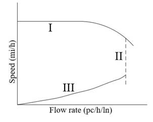
Fig. 1. Three-regime speed-flow model. Uncongested (I), queue discharge
(II)
and congested (III) regions [11]
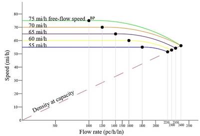
Fig. 2. Speed-flow rate relationship in basic freeway sections for
different free-flow speeds [13]
In
Figure 2, under uncongested traffic flow conditions, the curves consist of two
regions; the linear part and the concave part. The linear part is the
constant-speed portion of the curve and represents the free flow speed (FFS).
FFS is an important parameter as several conditions such as capacity, service
flow rates, daily service volumes and service volumes depend on it. In the
regions where the flow rate is higher, the speed starts to decrease, and it
shows a curvilinear change until it reaches the capacity value of the road
segment. The transition between the linear part and the concave part is
expressed as the BP.
The
model proposed in HCM [12] explains the
speed-flow relationship with curves as shown in Figure 2. The speed-flow
function is anchored by two points (BP, FFS) and (C, CS) that represent two
regions, while C and CS represent the capacity and the speed at capacity,
respectively. The basic approach of HCM [12] is quite
simple since these anchor points can be algebraically determined with given
equations. The equations require the estimation of deterministic values for BP,
FFS, C, and CS. In this regard, some researchers have analyzed the speed-flow
relationship to find BP. However, the proposed methods to find BP are
relatively complicated and computationally heavy [14, 15]. One simple
and effective approach using standard deviations of speed measurements was
offered by Roess [16]. This method
is based on the assumption that the standard deviation of speed is low for flow
values smaller than BP and begins to increase abruptly as flow is greater than
BP.
3.
EXPERIMENTS
3.1.
The dataset and features
Traffic
flow and speed data are obtained from the performance measurement system
(PeMS). PeMS is a freeway performance measurement system that supplies
historical and real-time data collected from detectors in freeways throughout
California [17]. The dataset
includes readings of a dual-loop detector in the California SR-17 freeway. Four
weeks of data from four different seasons of 2017 and 2018 (32 weeks of data in
total) were used. The original dataset involved speed and flow data collected for
5 minutes intervals. Therefore, three of these measurement intervals are
combined to obtain a dataset for 15 minutes intervals. This combination
procedure involves the calculation of total flow and average speed. Three
consecutive flow data are added to obtain the total flow. On the other hand,
the sum of speed data weighted by corresponding flow data is calculated for
average speed. Thus, one hour of data is represented by four examples.
The
features extracted from the dataset may be collected under two categories;
temporal features and measurement features. The temporal features are
categorical and they denote “hour of day” and “day of
week”. These features are represented by a one-hot encoding. Therefore,
the dimensions of corresponding binary vectors for these categorical features
are 24 and 7, respectively. The measurement features are continuous values and
involve current and historical data for flow and speed. The historical data
consists of measurements from one day before and one year before the time to be
predicted. Hence, three features (current, yesterday, and last year) for two
different measurements (speed and flow) are generated as a six-dimensional
feature vector. A representation of the feature vector is illustrated in Figure
3.
Fig. 3. Representation of a sample feature vector
3.2.
Speed and flow prediction
The
experiments involved in this work may be collected into three major groups.
First, for a prediction horizon of 15 minutes, speed and flow values are
predicted using four different machine learning methods. The next step starts
with generating speed-flow diagrams using the predicted values. These diagrams
provide useful information for detecting traffic conditions of the relevant
road segment. Therefore, the predicted values are used to calculate the BP
flow, which is an important parameter for traffic analysis and modeling. In the
final step, the state of the traffic is estimated by comparing the predicted
flow value with the BP flow calculated in the second step.
For
speed and flow prediction, the dataset is split into training and test sets
with proportions of 75 and 25%, respectively. To evenly distribute the seasonal
data into these sets, the first three weeks from each season are merged to
generate the training set and the following one-week data are merged to
generate the test set. Instead of training a model for the prediction of every
sample in the test set, only one model is sufficient to make predictions for
all data in the test set as the traffic speed and flow patterns have similar
structures throughout the day and week [18, 19].
Using
the MLPNN, SVR, GBDT, and kNN methods, four different models are trained and
tested on these sets. Relevant parameters for these models are selected using
10-fold cross-validation, and the corresponding prediction performance values
are provided in the results section.
It is important to note at this point that the speed and flow prediction
is an intermediate step to determining BP flow.
3.3. Determining breakpoint values
It
is critical to determine the first BP in the flow axis of the speed-flow
relationship. The speed values up to this BP are considered to be constant.
Hence, for the values greater than the BP, the speed values start to decrease
while flow increases. Thus, it may be concluded that the standard deviation of
speed value from the FFS increases after BP [16]. The use of
standard deviation is a common method for determining BP in the literature [6, 20].
BP
values using the actual (![]() ) and
predicted (
) and
predicted (![]() ,
, ![]() ,
, ![]() ,
, ![]() ) speed-flow
distributions are calculated separately through the standard deviation method
and the closeness of these BP values is observed. According to the standard
deviation analysis, the flow axis is divided into a set of equally-sized
ranges. Given a range, the corresponding standard deviation is calculated
through equation 1:
) speed-flow
distributions are calculated separately through the standard deviation method
and the closeness of these BP values is observed. According to the standard
deviation analysis, the flow axis is divided into a set of equally-sized
ranges. Given a range, the corresponding standard deviation is calculated
through equation 1:
|
|
(1) |

where ![]() is
the speed values of the samples in the range,
is
the speed values of the samples in the range, ![]() is the
free-flow speed for the site, and
is the
free-flow speed for the site, and ![]() is
the number of observations belonging to the range. The size of the ranges is
selected as 50 pc/15 min and the corresponding
is
the number of observations belonging to the range. The size of the ranges is
selected as 50 pc/15 min and the corresponding ![]() values are calculated for flow rates greater
than 200 pc/15 min.
values are calculated for flow rates greater
than 200 pc/15 min.
3.4. Estimating the state of traffic flow
Calculation
of BP flow allows the speed-flow space to be divided into two parts; stable and
metastable regions. Therefore, the samples with flow values smaller than the
calculated BP are estimated as “stable state”. The other samples
that have flow values higher than the calculated BP are labeled as
“metastable state”.
This
state estimation procedure is carried out on both the actual data and all
predictions. The labels obtained through comparing actual data with ![]() are considered as ground truth. State
estimation performance of each regression method is calculated by generating a
confusion matrix using the ground truth labels and estimated labels.
are considered as ground truth. State
estimation performance of each regression method is calculated by generating a
confusion matrix using the ground truth labels and estimated labels.
3.5. Performance metrics
To
evaluate the prediction performance of each machine learning method, four
different metrics commonly used in the literature are calculated. These metrics
are coefficient of determination (![]() ), root mean
squared error (RMSE), mean absolute percentage error (MAPE) and mean absolute
error (MAE). They are calculated as shown in equations 2-5 below:
), root mean
squared error (RMSE), mean absolute percentage error (MAPE) and mean absolute
error (MAE). They are calculated as shown in equations 2-5 below:
|
|
(2) |
|
|
(3) |
|
|
(4) |
|
|
(5) |

where ![]() and
and ![]() are actual and
predicted values for ith test sample,
are actual and
predicted values for ith test sample, ![]() is the mean value of all actual values in the
test set, n is the total number of samples in the test set.
is the mean value of all actual values in the
test set, n is the total number of samples in the test set.
As
for the performance of standard deviation method, first, ![]() is calculated using the actual target
values provided in the test set. Next,
is calculated using the actual target
values provided in the test set. Next, ![]() ,
, ![]() ,
, ![]() , and
, and ![]() , are calculated using the
prediction outcome of each individual method. The predicted
, are calculated using the
prediction outcome of each individual method. The predicted ![]() value giving the minimum residual with
value giving the minimum residual with ![]() is concluded to be superior to the
others.
is concluded to be superior to the
others.
To
determine the performance of flow state estimation, a confusion matrix is
generated by considering the correct predictions of the metastable state as
true positives (TP) and the stable state as true negatives (TN). False
positives (FP) and false negatives (FN) are defined as misclassifications of
stable and metastable states, respectively.
Using
the confusion matrix, the accuracy, specificity and sensitivity values are
calculated as specified by equations 6-8:
|
|
(6) |
|
|
(7) |
|
|
(8) |
4.
RESULTS AND DISCUSSION
4.1.
Results for speed and flow prediction
The parameters of the used prediction methods have a
direct impact on the performance. As stated earlier, 10-fold
cross-validation is applied to the training set and the parameters with the
best validation results are selected. The number of hidden units in the MLPNN
model is determined as 40. The model is trained with a learning rate of 0.0001
and the rectifier linear unit is used as the activation function. Performance
of the SVR model is evaluated on two separate models with different kernel
functions. The first one (SVR-RBF) uses the Gaussian radial basis function
(RBF) as the kernel. The regularization term (![]() ) and the threshold
term
) and the threshold
term
(![]() ) are selected as 100
and 0.1, respectively. In addition, the standard deviation (
) are selected as 100
and 0.1, respectively. In addition, the standard deviation (![]() ) for the RBF kernel is set to 0.027. A polynomial kernel with a degree
of 4 and a bias term of 1 is used
in the other SVR model (SVR-POLY). This polynomial model has the parameter
setting as
) for the RBF kernel is set to 0.027. A polynomial kernel with a degree
of 4 and a bias term of 1 is used
in the other SVR model (SVR-POLY). This polynomial model has the parameter
setting as ![]() and
and ![]() . The GBDT model,
trained with a learning rate of 0.1, contains 300 boosting steps and weak
learners with a maximum depth of 3.
. The GBDT model,
trained with a learning rate of 0.1, contains 300 boosting steps and weak
learners with a maximum depth of 3.
For the kNN method, ![]() is selected. The relevant prediction results for
speed and flow are provided in Tables 1 and 2.
is selected. The relevant prediction results for
speed and flow are provided in Tables 1 and 2.
Tab. 1.
Speed prediction results
|
|
MLPNN |
SVR-RBF |
SVR-POLY |
GBDT |
kNN |
|
|
0.8564 |
0.8534 |
0.8263 |
0.8458 |
0.8398 |
|
|
1.4956 |
1.5111 |
1.6448 |
1.5496 |
1.5793 |
|
|
0.0525 |
0.0514 |
0.0517 |
0.0507 |
0.0518 |
|
|
0.8298 |
0.7752 |
0.7996 |
0.7771 |
0.8290 |
Tab. 2.
Flow prediction results
|
|
MLPNN |
SVR-RBF |
SVR-POLY |
GBDT |
kNN |
|
|
0.9862 |
0.9850 |
0.9858 |
0.9839 |
0.9829 |
|
|
57.6910 |
60.1981 |
58.6689 |
62.3388 |
64.3020 |
|
|
2.7234 |
2.7147 |
2.7190 |
2.7151 |
2.7122 |
|
|
39.6470 |
40.8914 |
40.0278 |
42.5258 |
43.3346 |
As observed from the ![]() values
in both tables, the models are better at predicting traffic flows containing
less rapid changes than speed data. Among the predictive models, MLPNN has the
highest
values
in both tables, the models are better at predicting traffic flows containing
less rapid changes than speed data. Among the predictive models, MLPNN has the
highest ![]() and the lowest
and the lowest ![]() for both
cases. For speed prediction,
for both
cases. For speed prediction, ![]() of GBDT
and
of GBDT
and ![]() of
SVR-RBF are lower than the other methods by 0.0018 and 0.0546, respectively.
Similarly for flow prediction, the lowest values for
of
SVR-RBF are lower than the other methods by 0.0018 and 0.0546, respectively.
Similarly for flow prediction, the lowest values for ![]() and
and ![]() are
obtained by kNN and MLPNN, respectively. Actual data and predictions with MLPNN
for a one-day duration are given in Figure 4, while scatter plots of predicted
data versus actual data are provided in Figure 5. Majority of the predictions
with a higher error are in the low speed, high flow region. This is the region
belonging to the metastable traffic flow, and it corresponds to a relatively
small period of one-day timespan. Thus, the proportion of data related to the metastable
state is low indicating that the methods have limited learning on this state.
are
obtained by kNN and MLPNN, respectively. Actual data and predictions with MLPNN
for a one-day duration are given in Figure 4, while scatter plots of predicted
data versus actual data are provided in Figure 5. Majority of the predictions
with a higher error are in the low speed, high flow region. This is the region
belonging to the metastable traffic flow, and it corresponds to a relatively
small period of one-day timespan. Thus, the proportion of data related to the metastable
state is low indicating that the methods have limited learning on this state.
Although inspecting the quantitative results in
Tables 1 and 2 makes it possible to determine which method has a better
prediction performance, it may be difficult to draw a final conclusion about
the best method as the prediction results are very close to each other. Very
small standard deviation of ![]() values for speed (
values for speed (![]() ) and flow (
) and flow (![]() ) predictions are indicators for this.
) predictions are indicators for this.
|
(a) |
(b) |
|
Fig. 4. Actual data and MLPNN
predictions for: (a) speed, |
|
|
(a) |
(b) |
|
Fig. 5. Actual data and MLPNN
predictions for: (a) speed, |
|
4.2. Results
for BP calculation
The predictions made by the
machine learning methods are used to calculate the BP flow value. For this
purpose, the standard deviation method is applied to actual speed and flow data
as well as their predictions. The speed-flow distribution for actual data and
corresponding predictions with the MLPNN method is given in Fig. 6.
|
|
|
|
(a) |
(b) |
Fig. 6. Scatter plots of speed versus flow for: (a)
actual data and (b) MLPNN predictions
Calculating BP involves determining standard deviations of speed values
within specified flow ranges. ![]() value for standard deviation calculation is obtained
by averaging the speed values in the first flow portion (corresponding to 50
minimum flow values) [20]. To observe the change in standard deviation for
consecutive flow ranges, related plots for all prediction methods, as well as
the actual data, are generated (Figure 7). The BP is defined as the flow value
where there is a significant increase in the standard deviation. The smallest
flow value at which the first derivative of the standard deviation is greater
than 0.1 is determined as the BP. For all the predicted data and the actual
data, standard deviation analysis outputs identical BP (1050 pc/15 min).
value for standard deviation calculation is obtained
by averaging the speed values in the first flow portion (corresponding to 50
minimum flow values) [20]. To observe the change in standard deviation for
consecutive flow ranges, related plots for all prediction methods, as well as
the actual data, are generated (Figure 7). The BP is defined as the flow value
where there is a significant increase in the standard deviation. The smallest
flow value at which the first derivative of the standard deviation is greater
than 0.1 is determined as the BP. For all the predicted data and the actual
data, standard deviation analysis outputs identical BP (1050 pc/15 min).
4.3.
Results for state of flow estimation
The speed-flow distributions with calculated BP
levels are visualized for actual data and MLPNN predictions in Figure 8.
Quantitative results of estimation obtained with different methods are given in
Table 3. The state estimation accuracy is highest for the MLPNN method. On the
other hand, kNN and SVM-POLY methods have better specificity and sensitivity
values, respectively. This means that the rate of true positive estimations is
higher with SVM-POLY; hence, it is better at detecting metastable states. Conversely,
a high true negative rate for kNN means that this method is relatively more
successful than others in estimating the stable states of traffic. However, the
best overall accuracy is obtained via the MLPNN method, which has the highest ![]() value
for regression as well.
value
for regression as well.
The average flow of misclassified samples is 1050.62 pc/15 min and the
corresponding standard deviation is 77.01 pc/15 min. Therefore, it is possible
to conclude that majority of the misclassifications are in the vicinity of the
calculated BP.
Tab. 3.
Results for state of flow estimation
|
|
MLPNN |
SVM-RBF |
SVM-POLY |
GBDT |
kNN |
|
|
|
Accuracy |
0.9702 |
0.9649 |
0.9676 |
0.9608 |
0.9691 |
|
|
|
Specificity |
0.9704 |
0.9566 |
0.9618 |
0.9618 |
0.9731 |
|
|
|
Sensitivity |
0.9700 |
0.9712 |
0.9720 |
0.9602 |
0.9661 |
|
|
|
(a) |
(b) |
||||||
|
(c) |
(d) |
||||||
|
(e) |
(f) |
||||||

Fig. 7. Standard deviations versus flow for: (a) actual
data, (b) MLPNN,
(c) SVR-RBF, (d) SVR-POLY, (e) GBDT, (f) kNN predictions
5. CONCLUSIONS
In this work, a method to estimate the state of
traffic for 15 minutes ahead is proposed. In contrast with the majority of
related papers in which only speed or flow predictions are made, this method
involves predicting and further processing of both of these data. Using these
predictions, speed-flow diagrams are generated and then BP flow is calculated
as the separating threshold between two traffic states: stable and metastable.
As the final step, the predicted samples are labeled with one of these states
as the estimation of the traffic state. Although the highest prediction and
state estimation performance are obtained via the MLPNN method, the results
obtained through other methods are very close to it. Besides, BP flow values
calculated using the predicted values are all identical and they are also equal
to the BP flow calculated using the actual data. This indicates that speed and
flow predictions are capable of representing the state transition despite some
errors in the predictions.
The samples having lower speed and higher flow
values are related to the metastable state and the proportion of this data is
relatively small. Therefore, the patterns in the metastable data cannot be
learned well. Eventually, the error on the predictions of the samples of this
state is high. To eliminate the imbalance in the data, increasing the number of
samples belonging to the metastable state may be considered as a future work.
|
|
|
|
(a) |
(b) |
Fig. 8. Scatter plots showing the stable and metastable
regions for: (a) actual data
and (b) MLPNN predictions after BP calculation
Acknowledgment
The authors would like to thank Prof. Dr. Faruk
Fırat Çalım for his valuable support during this study.
References
1.
Bąkowski
Andrzej, Leszek Radziszewski. 2022. „Analysis of the Traffic Parameters
on a Section in the City of the National Road during Several Years of
Operation”. Communications - Scientific Letters of the University of
Zilina 24(1): 12-25. DOI: 10.26552/com.C.2022.1.A12-A25.
2.
Lendel Viliam, Lucia Pancikova, Lukas Falat,
Dusan Marcek. 2017. „Intelligent Modelling with Alternative Approach:
Application of Advanced Artificial Intelligence into Traffic Management”.
Communications - Scientific Letters of
the University of Zilina 19(4): 36-42. DOI: 10.26552/com.C.2017.4.36-42.
3.
Mohammad Mehdi Khabiri, Fatemeh Matin
Ghahfarokhi, Sara Sarfaraz, Hasan Mohammadi Anaie. 2022. „Application of
Data Mining Algorithm to Investigate the Effect of Intelligent Transportation
Systems on Road Accidents Reduction by Decision Tree”. Communications - Scientific Letters of the
University of Zilina 24(2): 36-45. DOI: 10.26552/com.C.2022.2.F36-F45.
4.
Ma X., Z. Tao, Y. Wang, H. Yu, Y.
Wang. 2015. "Long short-term memory neural network for traffic speed
prediction using remote microwave sensor data". Transportation Research
Part C: Emerging Technologies 54: 187-197. DOI: 10.1016/j.trc.2015.03.014.
5.
Greenshields B.D. 1935. "A study in highway
capacity". Highway Research Board Proc. 1935: 448-477.
6.
Elfar A., A. Talebpour, H.S. Mahmassani. 2018.
"Machine learning approach to short-term traffic congestion prediction in
a connected environment". Transportation Research Record 2672:
185-195. DOI: 10.1177/0361198118795010.
7.
Van Lint J. C. Van Hinsbergen. 2012.
"Short-term traffic and travel time prediction models". Artificial
Intelligence Applications to Critical Transportation Issues 22: 22-41.
8.
Özuysal M., S.
Çalışkanelli, S. Tanyel, T. Baran. Year. 2009. "Capacity
prediction for traffic circles: applicability of ANN". In: Proceedings of the Institution of Civil
Engineers-transport: 195-206. Thomas Telford Ltd.
9.
Zhang L., Q. Liu, W. Yang, N. Wei, D. Dong.
2013. "An improved k-nearest neighbor model for short-term traffic flow
prediction". Procedia-Social and Behavioral Sciences
96: 653-662. DOI: 10.1016/j.sbspro.2013.08.076.
10.
Castro-Neto M., Y.-S. Jeong, M.-K. Jeong, L.D.
Han. 2009. "Online-SVR for short-term traffic flow prediction under
typical and atypical traffic conditions". Expert systems with
applications 36: 6164-6173. DOI: 10.1016/j.eswa.2008.07.069.
11.
Hall F.L., V. Hurdle, J.H. Banks. 1993.
"Synthesis of recent work on the nature of speed-flow and flow-occupancy
(or density) relationships on freeways".
Transportation Research Record 1365:
12-18.
12.
HCM. Highway
Capacity Manual. 2000. Transportation Research Board of the National
Academies: Washington, D.C.
13.
HCM. Highway
Capacity Manual. 2010. Transportation Research Board of the National
Academies: Washington, D.C.
14.
Schoen J., A. May, W. Reilly, T. Urbanik. 1995.
"Speed-Flow Relationships for Basic Freeway Segments". Final
Report, NCHRP Project 3(45).
15.
Brilon W., M. Ponzlet. 1995. Applications of Traffic Flow Models, in Traffic and Granular Flow. World Scientific Publishing:
Jülich, Germany.
16.
Roess R.P. 2011. "Speed–Flow Curves
for Freeways in Highway Capacity Manual 2010". Transportation Research
Record: Journal of the Transportation Research Board 2257: 10-21.
17.
PeMS. Caltrans
Performance Measurement System. 2021. Available at: http://pems.dot.ca.gov/.
18.
Luo X., D. Li, Y. Yang, S. Zhang. 2019.
"Spatiotemporal traffic flow prediction with KNN and LSTM". Machine
Learning in Transportation 2019(Article ID 4145353).
19.
Soua R., A. Koesdwiady, F. Karray. 2016. "Big-data-generated
traffic flow prediction using deep learning and dempster-shafer theory". In:
International Joint Conference on Neural
Networks (IJCNN). IEEE. P. 3195-3202.
20.
Riente de Andrade G., J.R. Setti. 2014.
"Speed–Flow Relationship and Capacity for Expressways in
Brazil". Innovative Applications of the Highway Capacity Manual 2010 10.
Received 09.02.2022; accepted in
revised form 30.03.2022
![]()
Scientific Journal of Silesian University of Technology. Series
Transport is licensed under a Creative Commons Attribution 4.0
International License