Article
citation information:
Kądziołka, T., Opoka, K. Forecasting the number
of failures of the steering system components with the use of the grey system
theory method. Scientific Journal of
Silesian University of Technology. Series Transport. 2021, 112, 85-97. ISSN: 0209-3324. DOI: https://doi.org/10.20858/sjsutst.2021.112.7.
Tomasz
KĄDZIOŁKA[1],
Kazimierz OPOKA[2]
FORECASTING
THE NUMBER OF FAILURES OF THE STEERING SYSTEM COMPONENTS WITH THE USE OF THE
GREY SYSTEM THEORY METHOD
Summary. Steering systems are
one of the most important components of a car and have a direct impact on
safety and driving comfort. Therefore, high reliability is required of them.
One of the methods of object reliability estimation may be the grey system
theory. This method can be used not only to calculate the number of failures,
but also to calculate the wear of mating parts, and the vibrations of engines
and rolling elements. This work presents the use of the grey system theory for
the examination of motor vehicle steering system reliability. The forecast
number of failures was calculated for the various components of the steering
system and the grey system accuracy was assessed. This is aimed at finding out
how useful this theory is for forecasting the number of steering system
failures.
Keywords: steering mechanism, steering linkage, servo
system, reliability, grey system theory method
1. INTRODUCTION
The reliability theory in its field comprises the methods of failure
forecasting, detection of the laws affecting defects and the development of
ways of improving the reliability of objects. Forecasting object reliability is
a crucial issue in present times. It enables one to foresee the states of the
object in the future based on information on the states to have occurred
already. Forecasting permits the determination of machine maintenance or
inspection dates to ensure longer machine life and the operators’ or
travellers’ safety when the means of transport are under discussion.
Therefore, forecasting the future values of the symptoms of machinery technical
condition is an issue of importance that has been widely discussed in reference
literature [3, 17-20, 25]. One of the methods of object reliability assessment
is the grey system theory. It was initiated and described by the Chinese
scientist J.L. Deng in 1982 [5]. The theory is not only used in machine
condition forecasting but also in economics [3]. This method can be used to
calculate the number of failures, as well as to calculate the wear of mating
parts, and the vibrations of engines and rolling elements.
This article aims to forecast the number of failures of the selected
elements of the steering system of a selected motor vehicle using the
aforementioned method.
2. THE CHARACTERISTICS
AND OPERATIONAL CONDITIONS OF STEERING SYSTEMS
The steering system enables the driver to set, control and maintain the
required direction of the vehicle movement by the appropriate alignment of the
steered wheels. The steering system consists of three basic elements, that is,
the steering mechanism, the steering linkage and the servo system. The steering
mechanism consists of elements such as the steering wheel, steering column (the
housing and articulated steering wheel shaft), steering
gear and Pitman arm.
As mentioned above, the steering mechanism is used by the driver to set
the steered wheels at such an angle that the vehicle moves in the designated
direction. A typical steering system is shown in Figure 1 [7].
The steering wheel is made of a metal rod, polyurethane foam and fabric
or leather. It is important to select the steering wheel diameter properly so
that the force applied by the driver does not have to be too great. Generally,
the steering wheel diameter ranges from 450 [mm] for cars and 550 [mm] for
trucks and buses. Through special catches, fitted by pressing, is the airbag
assembly, placed in a plastic housing which usually functions as a horn
actuator. In cars with automatic transmission, the steering wheel may have
gear selection buttons; owing to them, the driver is not forced to take his or
her hands off the steering wheel, thus, comfort and safety are improved.
The steering column is designed to transmit torque from the steering
wheel to the steering gear. The steering column consists of a jacket attached
to the vehicle body and of a bearing-mounted steering wheel shaft. The shaft
top end is completed with a multi-spline, which is designed for fixing the
steering wheel, as well as with a thread for screwing the central clamp nut on.
The steering wheel shaft can be made as one whole or it can be sectional, that
is, consisting of two or three parts, connected by knuckle joints or
multi-splines.
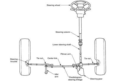
Fig. 1. The construction of the steering system [23]
The three-part steering wheel shaft consists of the upper and lower
shafts connected with each other by pins, and the intermediate shaft. The lower
intermediate shaft end, seated on a multi-spline, permits a change of its
length, and the two knuckle joints permit the change of the torque transmission
angle. A flexible joint is often placed between the lower end of the steering
wheel shaft or of the intermediate shaft to compensate for small angular
deviations and minimise vibrations transmitted to the steering wheel caused by
driving on rough roads. The steering column is equipped with additional
mechanisms; an energy absorption mechanism, steering wheel lock and adjustment
mechanisms (steering wheel tilt or overhang) [7].
The steering gear is the main steering mechanism unit that acts as a
reducer transmitting the rotary motion from the steering wheel to the steering
linkage. The task of the steering gear is to ensure the appropriate kinematic
and dynamic ratio so that the driver's effort is as low as possible.
Depending on the design details, transmission gears can be divided [7]:
those providing the output rotary motion (worm and nut, globoid as well as ball
and screw gear) and those providing the output translational motion (rack and
pinion gear).
The steering linkage is a set of rods and levers connecting the steered
wheels through the ball joints and Pitman arms. The task of the steering
linkage is to achieve a kinematic connection, causing the vehicle wheels to
move along a curvilinear track without skidding.
There are two types of steering linkage: one for the suspension with a
rigid front axle and one for independent suspension. In the case of a rigid
front axle, the steering linkage has a trapezoidal shape and a simple
structure; however, such linkages are subject to a kinematics error. The
independent suspension steering linkage should ensure the constant steered
wheel toe-in during an independent movement of one of the steered wheels of the
vehicle. The solution to this problem is the use of a central bar connecting
the two side rods: the left and right one. The trapezoidal steering linkage
with the steering gear providing output rotary motion comprises the following
elements: the central rod, side rods (right and left); rod support; Pitman arms
and stub axles (right and left).
In rack and pinion gears, the central rod is a toothed rack. The
triangle-shaped steering linkage with rack and pinion gear comprises: side rods
(right and left), Pitman arms and stab axles (right and left) [7].
The operation conditions to which the steering systems are subjected
cause frequent failures of the components within it. The assessment of the
technical condition of the steering system and the steering linkage pertains to
the steering column and wheel, the steering gear and the condition of the
steering rod ball joints.
The assessment is undertaken by checking the steering wheel lost motion
and clearance in the steering mechanisms. Steering wheel lost motion is the
result of excessive clearance in the steering system. Lost motion is assessed
using the LUZ-1 instrument, permitting the measurement of the “idle”
steering wheel rotation angle, which is the outcome of the total clearance of
the entire system. The permissible value of the angle with the wheels set to
drive straight ahead is 5-7° in cars and 15-29°
in trucks.
The following should be included among the typical kinds of failure of
the steering system:
- steering gear leakage,
- wear and tear of the mating elements of the steering gear,
- clearance in the ball joints of the rods,
- complete destruction of the ball joint (Figure 2),
- development of fatigue wear of cooperating elements.
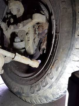
Fig. 2. An
example of complete destruction of a ball joint
The damage to the elements shown in Figure 2 may be the result of the
development of fretting wear. The condition for the development of this type of
wear is the occurrence of oscillating tangential displacements between
cooperating elements and the action of static forces [10, 13]. Fretting wear
occurs in many fields of technology and science. It is found, among others, in
rail vehicles [11, 12], aircraft components [2], as well as biotechnology [4].
3. RESEARCH METHODOLOGY
Input data needed for the analysis was obtained from a database
concerning the operation of a selected group of vehicles, and such has been
collected over the last ten years by the car repair shop where the vehicles
were serviced. Subject to analysis were the key elements of the steering
system, such as the servo pump, steering gear and steering rod ends. These
elements usually fail due to the condition of the road, and they directly
influence travellers’ safety.
By predicting the failure distribution trend, it is possible to
determine the point at which the failure threshold rises rapidly, and thus,
prevent the destruction of the system. This offers the option of ensuring
system protection and travellers’ safety, saving money.
4. CHARACTERISTICS OF THE GREY SYSTEM THEORY
The grey system theory is a relatively simple method as it does not
require complicated calculations [6, 8, 15, 22, 24].
Generally, the very name “grey system” shows the nature of the
method. It is an object’s operational stage in which an amount of
information (the number of failures) is known, and the other part is unknown.
The purely theoretical “grey system” theory model is
determined by differential equation (1) [1, 11, 24, 26]:
![]() (1)
(1)
The variables such as “a”
and “u” occurring in the
equation are calculated using matrix operators from the following equations
(2):
![]() ;
;
![]() (2)
(2)
Parameters B and Yn may be determined by
solving matrices (3) and (4):
 (3)
(3)
![]() (4)
(4)
The matrices come into being from the model input data. The outcome of
those mathematical operations is a two-line matrix a x u, which permits the determination of variables “a” and “u” which have been sought [9, 16].
The forecast values are calculated according to formula (5), which has
come into being by appropriate transformations:
![]() (5)
(5)
The determined parameters “a”
and ”u”
are substituted into the formula in which the initial value X(0) is equal to the first noted value.
The fact that the use of the method is reasonable may be determined by
several formula transformations, and then, the result compared with the values from
Table 1.
At the beginning, the remaining values are calculated based on formula
(6).
![]() (6)
(6)
Thereafter the arithmetic mean of the actual (noted) values is
calculated with the use of formula (7).
![]() (7)
(7)
The average of the remaining data q(k) is determined
based on formula (8).
![]() (8)
(8)
Parameters S1 and S2, that is, the variances of
the actual and remaining data are, in turn, determined based on formulae (9)
and (10).
![]() (9)
(9)
![]() (10)
(10)
The quotient of the values obtained based on the formula above is equal
to C:
![]() (11)
(11)
Now the method accuracy is checked by comparing the result with the
values in Table 1.
Tab. 1
The table permitting method accuracy
determination
|
Forecast accuracy |
P |
|
|
Good |
>0.95 |
<0.35 |
|
Satisfactory |
0.8-0.9 |
0.35-0.5 |
|
Unsatisfactory |
0.7-0.8 |
0.5-0.65 |
|
Poor |
<0.7 |
>0.65 |
5. FORECAST OF THE NUMBER OF FAILURES OF THE SELECTED STEERING SYSTEM
COMPONENTS
5.1. Steering gear
Input data in the form of the number of the noted steering gear failures
for specific mileage are collated in Table 2. Fifteen time intervals within
15,000-225,000 km have been indicated, in which the input data is noted in the
form of the number of recorded failures of the ten vehicles under observation.
The number of failures within the other five time intervals, that is, from
240,000 km to 310,000 km, are estimated based on the analysis.
Tab. 2
Schedule
of input data
|
Measurement |
1 |
2 |
3 |
4 |
5 |
6 |
7 |
8 |
9 |
10 |
|
Mileage [km] |
15000 |
30000 |
45000 |
60000 |
75000 |
90000 |
105000 |
120000 |
135000 |
150000 |
|
A |
35 |
37 |
41 |
49 |
56 |
69 |
77 |
85 |
93 |
101 |
|
Measurement |
11 |
12 |
13 |
14 |
15 |
16 |
17 |
18 |
19 |
20 |
|
Mileage [km] |
165000 |
180000 |
195000 |
210000 |
225000 |
240000 |
265000 |
280000 |
295000 |
310000 |
|
A |
113 |
129 |
134 |
141 |
160 |
- |
- |
- |
- |
- |
A – number of failures noted X0(i)
With the use of formulae (1)-(4), parameters B and Yn were
first determined, then parameters a and u needed for
the estimation of the number of failures were calculated.
![]()
![]()
The values of parameters a and u,
respectively, are as follows:
a = -0,101378
When all the unknown quantities are already known, the forecast number
of steering gear failures may be determined based on formula (5). The results
of those calculations are compiled in Table 3. The comparison of the number of
failures noted with the forecast number is shown in Figure 3.
The next stage of the calculations is the
determination of method accuracy. Formulas (6)-(11) will be used for this purpose. Parameter C has been determined, which will be
compared with Table 1. The obtained result is C=0.121725, which confirms that method accuracy is at a good level.
Tab. 3
Forecast number of steering gear failures
|
X'0(1) |
X'0(2) |
X'0(3) |
X'0(4) |
X'0(5) |
X'0(6) |
X'0(7) |
X'0(8) |
X'0(9) |
X'0(10) |
|
35 |
44.33 |
49.06 |
54.30 |
60.09 |
66.51 |
73.60 |
81.46 |
90.15 |
99.77 |
|
X'0(11) |
X'0(12) |
X'0(13) |
X'0(14) |
X'0(15) |
X'0(16) |
X'0(17) |
X'0(18) |
X'0(19) |
X'0(20) |
|
110.41 |
122.19 |
135.23 |
149.66 |
165.63 |
183.30 |
202.85 |
224.50 |
248.45 |
274.96 |
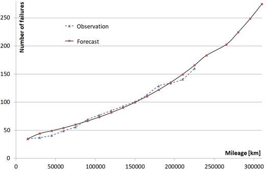
Fig. 3. The distribution of the noted and estimated number
of steering gear failures
5.2. Steering rod ends
Input data in the form of the number of the noted steering gear failures
for specific mileage are collated in Table 4. As in the previous case, fifteen
time intervals within 15,000-225,000 km were indicated, in which the input data
is noted in the form of the number of recorded failures of the ten vehicles
under observation. The number of failures within the other five time intervals,
that is, from 240,000 km to 310,000 km, are estimated based on the analysis.
Tab.
4
Schedule of initial values and mileage
|
Measurement |
1 |
2 |
3 |
4 |
5 |
6 |
7 |
8 |
9 |
10 |
|
Mileage [km] |
15000 |
30000 |
45000 |
60000 |
75000 |
90000 |
105000 |
120000 |
135000 |
150000 |
|
A |
45 |
48 |
50 |
61 |
73 |
86 |
94 |
101 |
115 |
124 |
|
Measurement |
11 |
12 |
13 |
14 |
15 |
16 |
17 |
18 |
19 |
20 |
|
Mileage [km] |
165000 |
180000 |
195000 |
210000 |
225000 |
240000 |
265000 |
280000 |
295000 |
310000 |
|
A |
136 |
148 |
159 |
166 |
172 |
- |
- |
- |
- |
- |
A – the
number of noted failures X0(i)
With the use of formulas (1)-(4), parameters B and Yn were
first determined, then parameters a and u needed for
the estimation of the number of failures were calculated.
![]()
![]()
The values of parameters a and u,
respectively, are as follows:
a = -0.0907
u = 50.96
When all the unknown quantities are already known, the forecast number
of failures of steering rod ends may be determined based on formula (5). The
results of the calculations are compiled in Table 5. The comparison of the
number of failures noted with the forecast number is shown in Figure 4.
Tab.
5
Forecast numbers of steering rod end failures
|
X'0(1) |
X'0(2) |
X'0(3) |
X'0(4) |
X'0(5) |
X'0(6) |
X'0(7) |
X'0(8) |
X'0(9) |
X'0(10) |
|
45 |
57.61 |
63.08 |
69.07 |
75.62 |
82.80 |
90.67 |
99.27 |
108.70 |
119.02 |
|
X'0(11) |
X'0(12) |
X'0(13) |
X'0(14) |
X'0(15) |
X'0(16) |
X'0(17) |
X'0(18) |
X'0(19) |
X'0(20) |
|
130.32 |
142.69 |
156.24 |
171.07 |
187.31 |
205.10 |
224.57 |
245.89 |
269.23 |
294.79 |
The next stage of the calculations is the determination of method
accuracy. Formulas (6)-(11) will be used for this purpose. Parameter C has been determined, which will be
compared with Table 1. The obtained result is C=0.161643, which confirms that method accuracy is at a good level.
5.2. Servo pump
Input data in the form of the number of the noted servo pump failures
for specific mileage are collated in Table 6. In this case, fifteen time
intervals within 15,000-225,000 km have been indicated as well, in which the
input data is noted in the form of the number of recorded failures of the ten
vehicles under observation. The number of failures within the other five time
intervals, that is, from 240,000 km to 310,000 km, are estimated based on the
analysis.
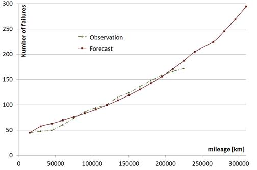
Fig. 4. The distribution of the noted and
estimated number of steering rod end failures
Tab. 6
Schedule of initial values and
mileage
|
Measurement |
1 |
2 |
3 |
4 |
5 |
6 |
7 |
8 |
9 |
10 |
|
Mileage [km] |
15000 |
30000 |
45000 |
60000 |
75000 |
90000 |
105000 |
120000 |
135000 |
150000 |
|
A |
20 |
28 |
37 |
44 |
56 |
62 |
69 |
73 |
81 |
90 |
|
Measurement |
11 |
12 |
13 |
14 |
15 |
16 |
17 |
18 |
19 |
20 |
|
Mileage [km] |
165000 |
180000 |
195000 |
210000 |
225000 |
240000 |
265000 |
280000 |
295000 |
310000 |
|
A |
96 |
107 |
110 |
115 |
121 |
- |
- |
- |
- |
- |
A – the number of noted failures X0(i)
With the use of formulae (1)-(4), parameters B and Yn were
first determined, then parameters a and u needed for
the estimation of the number of failures were calculated.
![]()
![]()
In this case, the values of parameters a and u, respectively, are as follows:
a= -0.08816
u= 38.27891
When all the unknown quantities are already known, the forecast number
of servo pump failures may be determined based on formula (5). The results of
the calculations are compiled in Table 7. The comparison of the number of
failures noted with the forecast number is shown in Figure 5.
Tab.
7
Schedule of initial values and
mileage
|
X'0(1) |
X'0(2) |
X'0(3) |
X'0(4) |
X'0(5) |
X'0(6) |
X'0(7) |
X'0(8) |
X'0(9) |
X'0(10) |
|
20 |
41.86 |
45.71 |
49.93 |
54.53 |
59.56 |
65.05 |
71.04 |
77.59 |
84.74 |
|
X'0(11) |
X'0(12) |
X'0(13) |
X'0(14) |
X'0(15) |
X'0(16) |
X'0(17) |
X'0(18) |
X'0(19) |
X'0(20) |
|
92.55 |
101.08 |
110.40 |
120.57 |
131.69 |
143.82 |
157.08 |
171.56 |
187.37 |
204.64 |
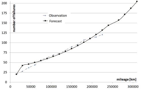
Fig. 5. The distribution of the noted and estimated number of servo pump
failures
The next stage of the calculations is the determination of method
accuracy. Formulas (6)-(11) are used for this purpose. Parameter C has been determined, which will be
compared with Table 1. The obtained result is C=0.191000, which confirms that method accuracy is at a good level.
6. CONCLUSION
The analysis aimed to assess the possible number of selected steering
system component failures that may occur as mileage increases.
Based on the method accuracy determination results, it may be believed
that the grey system analysis proposed in this article is suitable for
forecasting the number of steering system failures.
Moreover, system efficiency decreases with the distance covered by
vehicles. The question is about the number of the recorded failures, which
permits the relevant inspection cycles for the vehicles under analysis to be
designed. Based on the forecast, the number of possible system failures
increases proportionally. After covering 300,000 km, 275 various steering
gear failures, 295 steering rod failures and 205 servo pump failures should be
expected.
The considerations contained in the paper allows, among other things, to
increase road safety by forecasting possible damage to the steering systems and
repairing them in advance, before their complete destruction (Figure 2). By
analogous considerations, it is possible to predict damage to other mechanisms
or systems used not only in motor vehicles (braking system, drive system,
power-running system, drive unit) but also in working
machines as they can be used to predict their failure-free time operation and
precisely define the intervals between maintenance and repair.
References
1.
Bezuglov Anton,
Gurcan Comert. 2016. „Short-term freeway traffic parameter prediction: Application of grey system
theory models”. Expert Systems With Applications 62:
284-292.
2.
Bok-WonLee, Jungjun Suh, Hongchu Lee, Tae-gu Kim. 2011. „Investigations on fretting fatigue in
aircraft engine compressor blade”. Engineering Failure Analysis 18 (7):
1900-1908.
3.
Cempel
Czesław, Maciej Tabaszewski. 2007. „Application of grey system theory to modeling and
forecasting in machine condition monitoring”. Diagnostyka 2(42): 11-18.
4.
Chen-EnTsa, Jiames Hung, Youxin Hu, Da-Yung Wang, Robert M.Pilliar, Rizhi Wang. 2021. „Improving fretting corrosion resistance
of CoCrMo alloy with TiSiN and ZrN coatings for orthopedic applications”.
Journal of the Mechanical Behavior of
Biomedical Materials 114: 104233.
5.
Deng J-L. 1982. „Control Problems of Grey Systems”. Systems and Control Letters 1(5):
288-294.
6.
Deng Julong. 1989.
„Introduction to Grey System Theory”. The Journal of Grey System 1: 1-24.
7.
Gabryelewicz M.
2011. Podwozia i nadwozia pojazdów
samochodowych. [In Polish: Chassis
and bodies of motor vehicles]. Part
2. Warsaw: WKiŁ. ISBN: 9788320618266.
8.
Jui-Chen Huang. 2011.
„Application of grey system theory in telecare”. Computers in Biology and Medicine 41(5): 302-306.
9.
Kayacan Erdal, Ulutas Baris, Kaynak Okyay. 2010. „Grey system theory-based models in time series
prediction”. Expert Systems with Applications 37 (2):
1784-1789.
10.
Kowalski
Sławomir. 2018. „Analysis of
the possibilities of using CrN+a-C:H:W coatings to
mitigate fretting wear in push fit joints operating in rotational bending
conditions”. Tribologia 1:
45-55.
11.
Kowalski
Sławomir. 2016. „Application of dimensional analysis in the fretting wear studies”. Journal of the Balkan Tribological
Association 22(4-I):
3823-3835.
12.
Kowalski
Sławomir. 2020. „Failure analysis of the elements of a
forced-in joint operating in rotational bending conditions”. Engineering Failure Analysis 118: 104864.
13.
Kowalski
Sławomir. 2017. „Selected problems in the exploitation of wheel sets
in rail vehicles”. Journal of
Machine Construction and Maintenance 2: 109-116.
14.
Kowalski
Sławomir, Mariusz Cygnar. 2019.
„The application of TiSiN/TiAlN
coatings in the mitigation of fretting wear in push fit joints”. Wear 426: 725-734.
15.
Li-Qiang Hu,
Chao-Feng He, Zhao-Quan Cai, Long Wen, Teng Ren. 2018. „Track circuit fault prediction method
based on grey theory and expert system”. J. Vis.
Commun. Image R. 58: 37-45.
16.
Liu Sifeng. 2007.
„The Current Developing Status on Grey System Theory” The Journal of Grey System 2: 111-123.
17.
Maláková Silvia, Peter Frankovský, Daniela
Harachová, Vojtech Neumann. 2019. „Design of constructional
optimisation determined for mixed truck gearbox”. AD ALTA Journal of Interdisciplinary Research 9: 414-417. ISSN:
1804-7890.
18.
Maláková Silvia, Michal Puškár, Peter
Frankovský, Samuel Sivák, Maroš Palko, Miroslav Palko. 2020.
„Meshing Stiffness - A Parameter Affecting the Emission of
Gearboxes”. Applied Sciences
10(3): 1-12. DOI: 10.3390/app10238678.
19. Mazurkiewicz D. 2014. „Computer-aided
maintenance and reliability management systems for conveyor belts”. Eksploatacja i
Niezawodnosc – Maintenance and Reliability 16(3): 377-382.
20. Michalski R., S. Wierzbicki. 2008. „An
analysis of degradation of vehicles in operation”. Eksploatacja i
Niezawodnosc – Maintenance and Reliability 1: 30-32.
21.
Mu-Shang Yin.
2013. „Fifteen years of grey system theory
research: A historical review and bibliometric analysis”. Expert Systems with Applications 40:
2767-2775.
22.
Shuwei Wanga, Peng
Wanga, Yifei Zhang. 2020. „A
prediction method for urban heat supply based on grey system theory”. Sustainable Cities and Society 52: 101819.
23.
Steering and
suspancion components. Available at: https://en.tw-central.com.
24. Tabaszewski Maciej. 2014. “Prediction of
diagnostic symptom values using a set of models GM(1,1)
and a moving window method”. Diagnostyka
15(3): 65-68.
25.
Vaičekauskis
M., R. Gaidys, V. Ostaševičius. 2013. „Influence of boundary
conditions on the vibration modes of the smart turning tool”. Mechanika 3: 296-300.
26.
Xingqi Wang, Lei
Qi, Chan Chen, Jingfan Tang, Ming Jiang. 2014. „Grey System Theory based
prediction for topic trend on Internet”. Engineering Applications of Artificial Intelligence 29:
191-200.
Received 07.04.2021; accepted in revised form 23.06.2021
![]()
Scientific
Journal of Silesian University of Technology. Series Transport is licensed
under a Creative Commons Attribution 4.0 International License