Article
citation information:
Doğan, E. Performance analysis of
LSTM model with multi-step ahead strategies for
a short-term traffic flow prediction. Scientific
Journal of Silesian University of Technology. Series Transport. 2021, 111, 15-31. ISSN: 0209-3324. DOI: https://doi.org/10.20858/sjsutst.2021.111.2.
Erdem DOĞAN[1]
PERFORMANCE
ANALYSIS OF LSTM MODEL WITH MULTI-STEP AHEAD STRATEGIES FOR A SHORT-TERM
TRAFFIC FLOW PREDICTION
Summary. In this study, the
effect of direct and recursive multi-step forecasting strategies on the
short-term traffic flow forecast performance of the Long Short-Term Memory
(LSTM) model is investigated. To increase the reliability of the results, analyses
are carried out with various traffic flow data sets. In addition, databases are
clustered using the k-means++ algorithm to reduce the number of experiments.
Analyses are performed for different time periods. Thus, the contribution of
strategies to LSTM was examined in detail. The results of the recursive based
strategy performances are not satisfactory. However, different versions of the
direct strategy performed better at different time periods. This research makes
an important contribution to clarifying the compatibility of LSTM and
forecasting strategies. Thus, more efficient traffic flow prediction models
will be developed and systems such as Intelligent Transportation System (ITS)
will work more efficiently. A practical implication for researchers that
forecasting strategies should be selected based on time periods.
Keywords: traffic flow, LSTM, short-term prediction,
multi-step ahead strategies
1. INTRODUCTION
The significant increase in vehicle numbers and
travel demand raises traffic density on roads to critical levels. Proper
management of traffic flow can reduce this density. Today, this task is carried
out with smart systems operating under the Intelligent Transportation System
(ITS) and, these systems need information about future traffic conditions.
However, short-term traffic forecast is a challenging task of modern ITS.
Therefore, significant improvements are needed in developing a high-performance
traffic flow prediction model or improving existing models. Existing models can
be developed by optimising their parameters or using different forecasting
strategies.
The first study for the short-term traffic flow
prediction task was published in 1979 [1]. In the following years, parametric
and time series models were used for the prediction task [2-10]. The emergence of artificial
intelligence techniques such as Artificial Neural Networks (ANNs), Fuzzy Logic,
etc. accelerated the development of sophisticated short-term traffic prediction
models [11-14]. However, the exploding/vanishing
gradient problem of ANNs prevented the development of more advanced models in
the time series. Researchers overcome this problem with the Long Short-Term
Memory (LSTM) method developed in 1997 [15]. After this study, prediction
models based on the LSTM approach emerged.
LSTM is used in various fields, especially in
time series. Interestingly, LSTM was not utilised for traffic flow prediction
task until a study in 2016 [16]. Most studies on traffic flow
prediction in recent years aimed at developing a hybrid model with LSTM or compare
LSTM with other approaches. The LSTM model was improved with the k-nearest
neighbour (KNN) and compared with some state-of-art methods [17]. The developed model results were
slightly better than the standard LSTM model and significantly better than
other methods. Another study combined LSTM with an attention mechanism that
detects previous time steps that have a high impact on the current time step [18]. An LSTM model using temporary
information (T-LSTM) was developed [19]. Further, in the same study, T-LSTM
errors were compared with support vector machine, ARIMA and gated recurrent unit,
etc. approaches. The authors posit that the proposed technique increases LSTM's
prediction accuracy. A hybrid prediction model was developed using the graph
convolutional network and LSTM [20]. This hybrid model reduced errors
slightly compared to the traditional LSTM model.
LSTM's success in sequential data has motivated
researchers to do more study on the subject. Thus, LSTM was used for traffic
flow prediction tasks in a substantial number of studies. Generally, in these
studies, LSTM's traffic flow prediction performance was compared with other
methods, or its structure was updated to improve its performance, or a hybrid
model was developed using LSTM and other popular approaches. However, in these
studies, performance analysis of using a multi-step forecasting strategy with
LSTM for traffic flow prediction was not performed. Therefore, there is an
important research gap in this field. To close this important gap, this study
investigated which multi-step forecasting strategy works efficiently with an
LSTM model in the traffic flow prediction task. Thus, this study contributes to
developing high accuracy LSTM models for the traffic flow prediction task.
Three primary strategies and some of their
combinations were proposed in the literature for multi-step forecasting task.
These primary strategies are direct strategy based on developing a new model
for each step. A Recursive strategy that develops a single model and uses the
previous forecast value for each step in each step. Finally, a Multi-Input
Multi-Output (MIMO) strategy that developed only one model with the historical
data set and predicts the forecast horizon at once. Additionally, DirRec, the
combination of the direct and recursive strategy, and DirMo, the combination of the
direct and MIMO strategy [21]. Many studies in different fields
have been achieved with multi-step forecasting strategies [22-27]. However, most of the study results
are inconsistent about the proper strategy [21]. Furthermore, the fact that
different prediction problems have atypical features makes it difficult to solve
this inconsistency. Therefore, the issue of which strategy is good for which
problem is still completely unresolved. The investigation using different
forecasting strategies with LSTM in terms of the traffic flow prediction
problem, and the analysis of these results will contribute to the solution of
this inconsistency.
A few studies in the literature examined the
traffic flow prediction with a multi-step ahead strategy. Adaptive Kalman
filtering theory-based prediction models were proposed and compared with the
Gaussian Maximum likelihood and Constant and Heuristics Predictor approaches [28]. The models were tested for
forecasting horizons from 15 to 45 min. The forecast horizons examined are
short and only proportional performance criteria such as MAPE and APE were
utilised. Therefore, the long forecast horizon performances of the proposed
models have not been revealed. In addition, a one-way performance comparison is
another disadvantage of the study. A study using the spectral analysis and
statistical volatility model proposed a hybrid model. A one-step to ten-step
ahead forecasts of the models utilised were compared [29]. The proposed hybrid model
performance was compared with the ARIMA-GARCH model, and the hybrid model error
was reported to be fewer. Multi-step ahead strategies and gradient boosting
regression tree were used for the traffic speed prediction task [30]. Support vector regression was used
as the benchmark model and the researchers stated that the proposed model was
better. They similarly concluded that the DirRec strategy gave satisfactory
results for the short forecast horizon.
This article is divided into four sections. The
introduction covers the aim of this study and a literature review on the
subject. In the methodology section, the LSTM approach, the k-means++
algorithm, multi-step ahead forecasting strategies and the criteria used in
measuring errors are introduced. This is followed by the section where the
experimental results and the results are discussed. Finally, the
recommendations that emerged from this study and plans for further studies are
included in the conclusion.
2. METHODOLOGY
2.1. K-means++ and dropping similar datasets
Using various large datasets in a
study increases the reliability of the analysis results. However, analysis with
many similar data sets increases the cost of the analysis and its effect on the
results is limited. Excessive analysis can be avoided by dropping similar
datasets. Many traffic flow data sets were collected for this study. Therefore,
the procedure to reduce the number of datasets was applied. To extract similar
datasets, datasets were clustered according to their similarities. This process
was performed with the k-means++ algorithm according to the statistical
properties of the datasets.
The k-means is an unsupervised widely-used clustering algorithm that
clusters data sets according to their similarities [31]. The k-means++ is an advanced
version of the k-means algorithm and improves the quality of the final solution
[32]. Therefore, k-means++ was preferred
rather than the conventional k-means to cluster datasets in this study.
However, the traffic flow datasets are time-dependent and contain plenty number
of data samples. For k-means++ to be able to cluster more effectively, the
properties of this time series should be expressed with fewer features. Hence,
traffic flow data are expressed with common statistical estimators.
Let ![]() denote the sth traffic flow dataset, where M is the number of
observations,
denote the sth traffic flow dataset, where M is the number of
observations, ![]() . Then, the estimators are arithmetic
mean
. Then, the estimators are arithmetic
mean ![]() , standard deviation (
, standard deviation (![]() , maximum (max
, maximum (max ![]() ) and minimum (min
) and minimum (min![]() ) values of the dataset. Thus, the
estimator’s vector in Equation 1 expresses a data set using four
statistical estimators of the dataset.
) values of the dataset. Thus, the
estimator’s vector in Equation 1 expresses a data set using four
statistical estimators of the dataset.
The ![]() vectors are created for each
traffic data set and aggregated in set E. The E is the set of vectors and can
be expressed as
vectors are created for each
traffic data set and aggregated in set E. The E is the set of vectors and can
be expressed as ![]() , where N is the total number of datasets. Thus, the datasets are
arranged to be clustered by k-means++.
, where N is the total number of datasets. Thus, the datasets are
arranged to be clustered by k-means++.
The k-mean++ algorithm searches for centroids with a heuristic approach.
First, k-mean++ randomly selects a random observation and defines it as a first
centroid ![]() . Then, it calculates the Euler distances (d2) of each observation to
the
. Then, it calculates the Euler distances (d2) of each observation to
the ![]() . The new centroid is calculated with a probability ratio based on d2.
The algorithm repeats this process until it reaches the total number of
centroid (P). On the other hand, determining the appropriate P, that is, number
of clusters increases the reliability of the analysis. Gap statistics used in
this study is recommended as a superior method for estimating cluster numbers
and it forecasts the optimum P using the within-cluster sum of squares [33]. Finally, each
. The new centroid is calculated with a probability ratio based on d2.
The algorithm repeats this process until it reaches the total number of
centroid (P). On the other hand, determining the appropriate P, that is, number
of clusters increases the reliability of the analysis. Gap statistics used in
this study is recommended as a superior method for estimating cluster numbers
and it forecasts the optimum P using the within-cluster sum of squares [33]. Finally, each ![]() is assigned to a centroid
with probability computation.
is assigned to a centroid
with probability computation.
To avoid costly analysis, a certain upper limit (Ng) was determined for
the number of ![]() in the clusters. Thereafter,
Ng random elements were selected in each cluster and this set of elements was
named as the next generation of that cluster. Thus, the number of members in
each cluster decreased. This step provided the advantage of faster analysis.
in the clusters. Thereafter,
Ng random elements were selected in each cluster and this set of elements was
named as the next generation of that cluster. Thus, the number of members in
each cluster decreased. This step provided the advantage of faster analysis.
2.2. LSTM model structure
Recurrent Neural Network (RNN) is
the previous version of LSTM [34]. RNN's deficient performance in
solving the long-term dependencies problem is the motivation for the
development of LSTM. LSTM is a gradient-based method and consists of connecting
sequential LSTM units. LSTM units include structures such as input gate (i),
output gate (o), and forget gate (f) as illustrated in Figure 1 [15]. LSTM overcomes the problem of
long-term dependencies using these gates.
The connections between the
successive LSTM units and these are given in Figure 1. Let time be t.
Thus, the inputs of the LSTM unit at t are: The input vector (xt),
the cell state of the previous LSTM unit (Ct-1) and the
hidden state of the previous LSTM unit (ht-1). The unit has
two exits. These are: cell state (Ct) and hidden state (ht)
at t.
The first step to calculate the
outputs of an LSTM unit ate time t is the forget gate operation and it is
calculated by Equation 2. Let σ be the sigmoid function, W(f,i,c,o) be the network parameters
matrix, b(f,i,c,o) be the bias
matrices and ⊙ denotes the product operation.
The next step is to identify the new
information to be stored in the cell state. Therefore, the new candidate (![]() ) and the input gate it are calculated
using Equation 3-4.
) and the input gate it are calculated
using Equation 3-4.
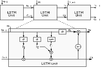
Fig. 1. Long short-term memory network unit
After these steps, Ct-1 is updated by using the ft,
it and ![]() in Equation 5.
in Equation 5.
The output gate (ot) is the process that
determines the parts of the cell state that will be in the output and can be
written as:
The other output of the LSTM unit, ht,
is calculated using Equation 7.
2.3. Multi-step forecasting strategies
Let
H be the prediction horizon and M be the number of observations.
Thus, multi-step prediction is the developing of a model using a series
composed of M observation [x1,
..., xM], and estimating the next H values [xM+1, ..., xM+H] of the
series with the developed model. This section presents three different
multi-step forecasting strategies for forecasting traffic flow.
Assume that an
untrained LSTM model is ![]() . First, the
. First, the ![]() is trained with
is trained with ![]() and becomes a trained LSTM model (
and becomes a trained LSTM model (![]() ). Subsequently, the
steps in the forecasting horizon are predicted using Equation 8.
). Subsequently, the
steps in the forecasting horizon are predicted using Equation 8.
![]()
where, t is
the current time, ![]() is the current time traffic flow and
is the current time traffic flow and ![]() is the one- step ahead prediction from t.
is the one- step ahead prediction from t.
2.3.2.
Direct strategy 2
Direct strategy-2
(Dir-2) is based on the principle of updating the model with the current
observation at each step and the prediction of the next step with the updated
model. Let Lh be the untrained LSTM model, where ![]() , where H is
the forecasting horizon. In the first step, Lh is trained
with the training set
, where H is
the forecasting horizon. In the first step, Lh is trained
with the training set ![]() and becomes
and becomes ![]() . Thus, the
prediction value for h = 1 will be written as
. Thus, the
prediction value for h = 1 will be written as ![]() . Other horizon
predictions are calculated by Equation 9 while
. Other horizon
predictions are calculated by Equation 9 while ![]() .
.
Direct strategy-1 (Dir-1) updates the model at every step. Thus, the
prediction speed of the model increases. However, as the size of the
forecasting horizon increases, forecast error increment probability Dir-1 may
increase.
Assume that the untrained LSTM model is ![]() . First, the
. First, the ![]() is trained with
is trained with ![]() and becomes a trained LSTM
model (
and becomes a trained LSTM
model (![]() ). Subsequently, the steps in the forecasting horizon are predicted by
using Equation 10.
). Subsequently, the steps in the forecasting horizon are predicted by
using Equation 10.
![]()
DS requires the updating of
every step of the model state, that is, the LSTM network state is updated with ![]() or
or ![]() in each step. This approach
may result in accurate forecasts. On the other hand, training the model with
new values in each step is an expensive approach in terms of calculation time.
Let Tso be the computational time. Thus, DS requires a
computational time of H x Tso for H steps [35]. Although DS requires a large computation time, it has been used with a
variety of learning and optimisation algorithms. For example, neural networks [24, 36] and extreme gradient boosting [27], whale optimisation algorithm [22], gradient boosting regression tree [30, 37], etc.
in each step. This approach
may result in accurate forecasts. On the other hand, training the model with
new values in each step is an expensive approach in terms of calculation time.
Let Tso be the computational time. Thus, DS requires a
computational time of H x Tso for H steps [35]. Although DS requires a large computation time, it has been used with a
variety of learning and optimisation algorithms. For example, neural networks [24, 36] and extreme gradient boosting [27], whale optimisation algorithm [22], gradient boosting regression tree [30, 37], etc.
2.3.3.
Direct-Recursive strategy
Direct-Recursive strategy (DirRec) is based on
the combination of direct and recursive strategies. First, a model is created
with available observation data in the direct and recursive strategy. Next,
predictions are made one step ahead. In each step, the previous model
prediction is used in the model to make predictions of future values. Similar
to Dir-2, ![]() is trained using the Tr and
is trained using the Tr and ![]() is formed after training. At each step, the LSTM network state is
updated with
is formed after training. At each step, the LSTM network state is
updated with ![]() , i.e.,
, i.e., ![]() . Equation 11 presents the inputs used in the
prediction in h=1 and h>1 stage.
. Equation 11 presents the inputs used in the
prediction in h=1 and h>1 stage.
![]()
The plurality of noise in the dataset can
increase model errors in prediction jobs with large H. Therefore, keeping
the forecast horizon short may be to the advantage of this method. The number
of studies using DirRec is limited [38-40], thus, there is potential for further
studies.
2.4. Error criteria and
forecast horizon periods
The errors of the strategies used in the dataset were evaluated with
three performance criteria. These are Mean Absolute Percentage Error (MAPE),
Mean Squared Error (MSE) and Root Mean Squared Error (RMSE), which are
frequently used to analyse model error. The equations of the criteria are in
Equations 11-13.


To determine the overall error trend of multiple data sets, the average
errors of all data sets were calculated for the error criteria by dividing
Equations 11-113 to N. Where, ![]() is the actual traffic flow,
is the actual traffic flow, ![]() is the forecasting value, N is the number of datasets. The RMSE
difference between the errors of Dir-1 and Dir-2 strategies was calculated
using Equation 14.
is the forecasting value, N is the number of datasets. The RMSE
difference between the errors of Dir-1 and Dir-2 strategies was calculated
using Equation 14.
![]()
LSTM errors were calculated separately for three predefined time periods,
to better understand the behaviour of the strategies within the forecast
horizon. Let xt be the current time traffic flow, thus,
traffic flow set for Period 1
can be written as ![]() where, HP1
is forecasting horizon of the P1. Furthermore, the traffic flow sets
for Period 2 and Period 3 can be written as,
where, HP1
is forecasting horizon of the P1. Furthermore, the traffic flow sets
for Period 2 and Period 3 can be written as, ![]() and
and ![]() , respectively.
, respectively.
3.
EXPERIMENTAL SETUP
This section concerns data set and model training pre-treatments. First,
information was given about the analysed datasets. Then, clustering of data
sets with the k-means algorithm was discussed. Hyperparameters used in the
training step of the LSTM model are given.
3.1. Data and data set clustering
A large number of data sets were used to analyse the result of using LSTM
with different forecasting strategies. This dataset requirement was met from
the PeMS database [41]. The PeMS database consists of information transmitted from detectors
located on highways in the state of California. Researchers can easily obtain
raw traffic data or processed data.
Care was taken to ensure that the datasets used in this study were
up-to-date, statistically different.
In addition, months in which the demand for travel increased were
considered for better interpretation of model errors. For this reason,
k-means++ analyses were made for 472 main lane data sets obtained from May to
August 2018. Lane traffic with different features, for example,
on-ramp/off-ramp, conventional highway lane, etc., were not used for the
analysis. Because different traffic patterns of these roads may decrease the
model performance.
Development and training of LSTM models for each data set consume
considerable computation time. To reduce the computation time, statistically
similar datasets were clustered with the k-means++ algorithm [32] and 20 datasets were randomly selected from these clusters for further
analysis. k-means++ can avoid some weak clusters found by the standard
k-mean algorithm. In addition, k-means ++ is frequently used for clustering in
studies in many different fields [42-45]. Hence, k-means++ was preferred to cluster the datasets.
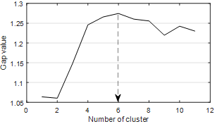
Fig. 2. Gap values for different number of clusters
The performance of a clustering algorithm increases due to determining
the optimal number of clusters for the problem. Therefore, various methods, for
example, Davies-Bouldin,
Calinski-Harabasz, Gap Statistic, Silhouettes [46-49] have been developed to select the optimum number of clusters. The gap
statistic method can be used with any distance metric and is defined even for
only one set [50], so it was preferred for this study. Gap statistic calculates a variable
named gap value for different cluster numbers, and the number of clusters with
the largest gap value is the best solution. The best cluster number for this
study is “6” and this number was determined from Figure 2,
which shows the result of gap statistics.
After determining the best number of clusters, 482 data sets were
clustered into 6 clusters using k-means++. Thus, similar data sets were
collected in the same cluster. Then, 20 data sets from each set were randomly
selected. The scattering of all and selected datasets according to average and
standard deviation values is given in Figure 3. The datasets of each cluster
are coloured in Figure 4 for better visualisation. This step is expected to
have affected the study result. However, this effect is extremely low since it
contains samples from all clusters. However, the modelling and analysis speeds
were increased significantly.
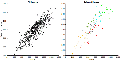
Fig. 3. Mean and standard deviation scatter plots for all and selected
data sets
Tab. 1.
Average descriptive statistics of the clusters
|
Cluster |
Part |
Mean |
Std |
Min |
25% |
50% |
75% |
Max |
|
C1 |
Train |
885 |
475 |
93 |
410 |
990 |
1275 |
1774 |
|
Test |
902 |
478 |
117 |
437 |
1037 |
1293 |
1723 |
|
|
C2 |
Train |
704 |
310 |
134 |
434 |
740 |
899 |
1950 |
|
Test |
695 |
290 |
224 |
436 |
754 |
895 |
1378 |
|
|
C3 |
Train |
371 |
224 |
23 |
157 |
392 |
534 |
1006 |
|
Test |
383 |
224 |
48 |
171 |
406 |
539 |
962 |
|
|
C4 |
Train |
682 |
359 |
84 |
331 |
760 |
961 |
1401 |
|
Test |
705 |
369 |
99 |
350 |
813 |
991 |
1352 |
|
|
C5 |
Train |
690 |
396 |
31 |
307 |
741 |
996 |
1656 |
|
Test |
708 |
412 |
62 |
302 |
777 |
1027 |
1553 |
|
|
C6 |
Train |
1044 |
522 |
135 |
499 |
1199 |
1497 |
1931 |
|
Test |
1070 |
517 |
206 |
544 |
1263 |
1509 |
1848 |
To demonstrate that the data sets used are multifarious, the average
statistical properties of the data sets in the clusters are summarised in Table
1. For the training stage of the LSTM models, 90% of the observations in the
data sets were reserved. The remaining 10% was used during the testing phase.
In Table 1, the statistical characteristics of these observations are given
separately. Thus, patterns can be discussed between LSTM model errors and these
statistical properties.
3.2. LSTM model and parameters
The LSTM and other layers in the deep learning network architecture used
in this study are illustrated in Figure 4. The network consists of input and
output layers and four other hidden layers. The LSTM layer is located after the
input layer. The network output
value is calculated using a regression layer.
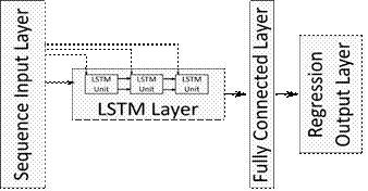
Fig. 4. Deep learning network architecture and LSTM layer
Determining the proper network structure and
parameters affects the predictive performance of the network. In particular,
the number of LSTM units significantly affects performance. Consequently,
experiments were carried out to determine the proper number of units for each
data set. In each experiment, models were developed by trying the number of
units between 5 and 250. Afterwards, the models with the lowest prediction
error were determined for comparison. Adam optimisation algorithm, widely
accepted for deep learning applications, was used [51].
The maximum number of epochs is
set to 250. The gradient threshold value was set to "1" in LSTM
training. The initial learning rate was determined as 0.005 and the learning
rate value was decreased by multiplying the learning rate by 0.2 in every 125
years. Before starting the model training, the data set was standardised for a
better fit with zero mean and unit variance. Fully connected layer output size
is set to 50 and fixed for all trials
4.
COMPARISON OF STRATEGY PREDICTION ERRORS
Traffic flow prediction errors of
LSTM models using different prediction strategies are statistically analysed in
this section. In addition, the prediction errors of the models for different
time periods determined for this study were compared. Thus, the impact of a
strategy on errors was more clearly analysed for different forecast horizons.
The errors of the strategy predictions are summarised
in Table 2 according to the error criteria and periods described in Section 2.4. The lowest and
highest outliers were removed from the dataset prediction errors and analyses
were performed for the remaining values. The DirRec strategy errors are
significantly higher than others. For example, DirRec all MAPE and RMSE are
about 4 times and all MSE is about 9 times more than other strategy criteria.
This result leads to the conclusion that no apparent advantage exists in
utilising the DirRec strategy for traffic flow prediction. Therefore, the
DirRec strategy was not discussed further.
The "All" line of Table 2 states that the errors of Dir-1 and
Dir-2 strategies are close to each other, however, on average, the performance of Dir-2 is a little more
advanced. The period errors in the table clearly reveal the superiority of
Dir-2 for P1 over Dir-1. However, this advantage is limited for P2 and P3. In
fact, Dir-1's MAPE value for P3 is lower than Dir-2 MAPE. This result suggests
that the Dir-1 might have some advantages in predicting the lower traffic flows
in distant forecasting horizon.
To visualise the results of Table 2,
the actual traffic flow and strategy predictions for station No: 312865 are shown in Figure 5 for the P1 period. The DirRec
predictions are less accurate than other strategies, and they can be easily
determined from the shape. In addition, Figure 5 confirmed that the other two
strategies have close predictions.
Tab. 2.
Mean errors of forecasting
strategies for periods
|
Forecasting Periods |
Dir-1 |
Dir-2 |
DirRec |
||||||||
|
|
|
|
|
|
|
|
|
|
|||
|
P1 ( |
11.11 |
70.6 |
5655 |
8.13 |
50.5 |
2987 |
26.69 |
156.8 |
30271 |
||
|
P2 ( |
8.62 |
53.5 |
3268 |
8.27 |
52.6 |
3220 |
29.40 |
149.4 |
27385 |
||
|
P3 ( |
8.91 |
59.2 |
3886 |
9.07 |
58.1 |
3773 |
29.73 |
178.1 |
35758 |
||
|
All |
9.31 |
61.1 |
4269 |
9.28 |
53.8 |
3327 |
43.33 |
161.4 |
31138 |
||
The ΔRMSE is calculated by
Equation 15 and the distributions of ΔRMSE are given in Figure 6. Due to
the poor results, DirRec is not considered here. The negative and the positive
ΔRMSE indicate that Dir-2 and Dir-1 have a low error, respectively. The
ΔRMSE is positive in 9 out of 120 datasets in P1. Therefore, Dir-1 has lower
RMSE for these 9 datasets. Dir-2 has a lower RMSE in the remaining 111
datasets.
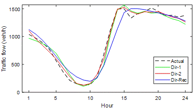
Fig. 5.
Comparison of multi-step ahead strategy predictions for P1 (Station No: 312865)
Conclusively, using Dir-2 in the
short prediction horizon, that is, P1, provides an important advantage. On the
other hand, P2's ΔRMSE number greater than zero and less than zero is
close to each other. This proximity likewise occurs for P3 and becomes more
concentrated around 0. Consequently, the use of Dir-2 is advantageous for P1,
and in other periods, the two strategies have no significant superiority over
each other.
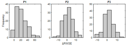
Fig. 6.
ΔRMSE distributions of Dir-1 and Dir-2 strategies for time periods
The errors in low value observations
have a high effect on MAPE. Therefore, it is suitable for analysing
performances in low traffic flows. In Figure 7, MAPE values of Dir-1 and Dir-2
are presented using box diagrams. In P1, Dir-1's highest MAPE is around 23% and
lowest MAPE around 5%. On the other hand, when outliers are not considered,
Dir-2 has MAPEs in the range of 15 to 3%. It can also be seen from the box plot
that 50% of Dir-1 MAPE measurements are between 7 and 14%. However, 50% of
Dir-2 MAPE measurements are between 6 and 9%. Hence, Dir-2 predicts low traffic
flows more successfully than Dir-1 in P1.

Fig. 7.
MAPE boxplots of Dir-1 and Dir-2 for time periods
In P2, the MAPE values of the two
strategies are close to each other. However, one of the outliers of Dir-1 has
35% MAPE. Therefore, MAPE value of Dir-1 in Table 2 is higher than Dir-2. Box
and box moustaches in P3 indicate that Dir-2 is slightly better than Dir-1 as
well, however, one of the outliers of Dir-2 has a MAPE value of 50%. Therefore,
in Table 2, it turns out that Dir-1 is better in terms of average MAPE.
However, Dir-2 shows better performance for the majority number of the data
sets.
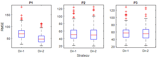
Fig. 8.
RMSE boxplots of Dir-1 and Dir-2 for time periods
Figure 8 shows the RMSE of
strategies. The RMSE criterion punishes relatively large errors more.
Therefore, it is a suitable criterion for comparing predictions that strategies
have high errors. The superiority of Dir-2 in P1 is clear in the RMSE
criterion. However, there are interesting results for other periods. Although
the RMSE distribution in P2 is close, the upper moustache of the Dir-1 has an
RMSE value of around 90, while the Dir-2s are around 100, meaning that the RMSE
of Dir-2 is higher. Less error in Dir-1 is observed in P3 too. Regarding high
error predictions, Dir-2 is clearly superior to Dir-1 in P1; however, Dir-1 has
slightly better performance than Dir-2 in P2 and P3.
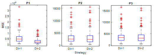
Fig. 9.
MSE boxplots of Dir-1 and Dir-2 for time periods
MSE is a suitable criterion for
evaluating a model's ability to predict unexpected values. In Figure 9 and P1,
MSE values of Dir-2 are significantly lower than Di-1. In the box diagrams for
P2 and P3, Dir-2 errors are slightly more than Dir-1. This situation is similar
to RMSE results. On the other hand, the number of outliers in MSE is higher
than other criteria. This indicates that both strategies are likely to make
extremely high errors for some observations.
Analysis results show that traffic
flow predictions of the LSTM and DirRec strategy have significantly higher
errors. On the other hand, Dir-2 is the best strategy for P1 compared to Dir-1
and DirRec. For P2 and P3, the Dir-1 strategy may be preferred, although Dir-2
seems better on average.
4. CONCLUSION
In this study, the capabilities of
the LSTM model were investigated with various numerous datasets for the traffic
flow prediction task. To our knowledge, this study is the first that proves the
effect of using different multi-step ahead forecasting strategies on the LSTM
performance. The modelling and analyses show that it is not proper to use the
DirRec strategy together with LSTM in traffic flow prediction. Further, for the
near future parts of the forecast horizon (P1), choosing Dir-2 makes a less
average error than the Dir-1 strategy. However, for the middle and distant
parts of the forecast horizon, using the Dir-1 strategy can be helpful. The
results obtained here may have implications for understanding the LSTM traffic
flow prediction performance tendency. Thus, more efficient approaches can be
developed for certain systems, for example, TMS and ITS. There are various
strategies in the literature. Despite the success shown, an important
limitation is the examination of only some of these various strategies.
Conducting further studies that include other strategies will advance
information on the subject. Consequently, researchers should be aware of the
fact that different forecasting strategies can improve LSTM performance
significantly and vice versa.
References
1.
Ahmed M.S., A.R. Cook. 1979. "Analysis of Freeway
Traffic Time-Series Data by Using Box-Jenkins Techniques". Transportation
Research Record. DOI: 10.3141/2024-03.
2.
Nagel K., M. Schreckenberg. 1992. "A cellular automaton
model for freeway traffic". Journal de Physique I. DOI:
10.1051/jp1:1992277.
3.
Cremer M. 1995. "On the calculation of individual travel
times by macroscopic models". Pacific Rim TransTech Conference. Vehicle
Navigation and Information Systems Conference Proceedings. 6th International
VNIS. A Ride into the Future. IEEE; 1995. P. 187-193. DOI:
10.1109/VNIS.1995.518837.
4.
Williams B.M. 2001. "Multivariate vehicular traffic flow
prediction: Evaluation of ARIMAX modeling". Transportation Research
Record. DOI: 10.3141/1776-25.
5.
Wu C.H., J.M. Ho, D.T. Lee. 2004. "Travel-Time
Prediction With Support Vector Regression". IEEE Transactions on
Intelligent Transportation Systems 5(4): 276-281. DOI:
10.1109/TITS.2004.837813.
6.
Audu Akeem A., Olufemi F. Iyiola, Ayobami A. Popoola, Bamiji
M. Adeleye, Samuel Medayese, Choene Mosima, Nunyi Blamah. 2021. "The
application of geographic information system as an intelligent system towards
emergency responses in road traffic accident in Ibadan". Journal of Transport and Supply Chain
Management 15(a546): 1-17. ISSN 2310-8789.
7.
Paľo Jozef, Ondrej Stopka. 2021. "On-Site Traffic
Management Evaluation and Proposals to Improve Safety of Access to
Workplaces". Communications
23(3): A125-A136. University of Zilina.
8.
Hossan Sakhawat, Naushin Nower. 2020. "Fog-based dynamic
traffic light control system for improving public transport". Public Transport 12: 431-454.
9.
Danilevičius
Algimantas, Marijonas Bogdevičius, Modesta Gusarovienė, Gediminas
Vaičiūnas, Robertas Pečeliūnas, Irena
Danilevičienė. 2018. “Determination of Optimal Traffic Light
Period Using a Discrete Traffic Flow Model”. Mechanika 24(6):
845-851.
10. Pranevičius
Henrikas, Tadas Kraujalis. 2012. "Knowledge based traffic signal control
model for signalized intersection". Transport
27(3): 263-267.
11. Zhong
M., S. Sharma, P. Lingras. 2005. "Short-Term Traffic Prediction on
Different Types of Roads with Genetically Designed Regression and Time Delay
Neural Network Models". Journal of Computing in Civil Engineering 19(1):
94-103. DOI: 10.1061/(ASCE)0887-3801(2005)19:1(94).
12. Smith
B.L., B.M. Williams, R. Keith Oswald, R.K. Oswald. 2002. "Comparison of
parametric and nonparametric models for traffic flow forecasting". Transportation
Research Part C: Emerging Technologies 10(4): 303-321. DOI:
10.1016/S0968-090X(02)00009-8.
13. Kamarianakis
Y., P. Prastacos. 2003. "Forecasting Traffic Flow Conditions in an Urban
Network: Comparison of Multivariate and Univariate Approaches". Transportation
Research Record 1857(1): 74-84. DOI: 10.3141/1857-09.
14. Kumar
B. Anil, Vivek Kumar, Lelitha Vanajakshi, Shankar C. Subramanian. 2017.
"Performance Comparison of Data Driven and Less Data Demanding Techniques
for Bus Travel Time Prediction". European Transport \ Trasporti Europei 65(9): 1-17. ISSN 1825-3997.
15. Hochreiter
S., J. Schmidhuber. 1997. "Long Short-Term Memory". Neural
Computation 9(8): 1735-1780. MIT Press Journals. DOI:
10.1162/neco.1997.9.8.1735.
16. Fu
R., Z. Zhang, L. Li. 2016. "Using LSTM and GRU neural network methods for
traffic flow prediction". 31st Youth Academic Annual Conference of
Chinese Association of Automation (YAC). IEEE. P. 324-328.
17. Luo
X., D. Li, Y. Yang, S. Zhang. 2019. "Spatiotemporal traffic flow
prediction with KNN and LSTM". Journal of Advanced Transportation.
Hindawi.
18. Yang
B., S. Sun, J. Li, X. Lin, Y. Tian. 2019. "Traffic flow prediction using
LSTM with feature enhancement". Neurocomputing 332: 320-327.
Elsevier B.V. DOI: 10.1016/j.neucom.2018.12.016.
19. Mou
L., P. Zhao, H. Xie, Y. Chen. 2019. "T-LSTM: A Long Short-Term Memory
Neural Network Enhanced by Temporal Information for Traffic Flow
Prediction". IEEE Access 7: 98053-98060. DOI:
10.1109/ACCESS.2019.2929692.
20. Li
Z., G. Xiong, Y. Chen, Y. Lv, B. Hu, F. Zhu, et al. 2019. "A Hybrid Deep
Learning Approach with GCN and LSTM for Traffic Flow Prediction". IEEE
Intelligent Transportation Systems Conference (ITSC). P. 1929-1933. DOI:
10.1109/ITSC.2019.8916778.
21. Ben
Taieb S., G. Bontempi, A.F. Atiya, A. Sorjamaa. 2012. "A review and
comparison of strategies for multi-step ahead time series forecasting based on
the NN5 forecasting competition". Expert Systems with Applications
39(8): 7067-7083. Elsevier Ltd. DOI: 10.1016/j.eswa.2012.01.039.
22. Du
P., J. Wang, W. Yang, T. Niu. 2018. "Multi-step ahead forecasting in
electrical power system using a hybrid forecasting system". Renewable
Energy 122: 533-550. DOI: https://doi.org/10.1016/j.renene.2018.01.113.
23. Papacharalampous
G., H. Tyralis, D. Koutsoyiannis. 2019. "Comparison of stochastic and
machine learning methods for multi-step ahead forecasting of hydrological
processes". Stochastic environmental research and risk assessment
33(2): 481-514. Springer.
24. Wang
J., J. Heng, L. Xiao, C. Wang. 2017. "Research and application of a
combined model based on multi-objective optimization for multi-step ahead wind
speed forecasting". Energy 125: 591-613. DOI:
https://doi.org/10.1016/j.energy.2017.02.150.
25. Guermoui
M., F. Melgani, C. Danilo. 2018. "Multi-step ahead forecasting of daily
global and direct solar radiation: a review and case study of Ghardaia
region". Journal of Cleaner Production 201: 716-734. Elsevier.
26. Wang
D., H. Luo, O. Grunder, Y. Lin, H. Guo. 2017. "Multi-step ahead
electricity price forecasting using a hybrid model based on two-layer
decomposition technique and BP neural network optimized by firefly
algorithm". Applied Energy 190: 390-407. Elsevier.
27. Xue
P., Y. Jiang, Z. Zhou, X. Chen, X. Fang, J. Liu. 2019. "Multi-step ahead
forecasting of heat load in district heating systems using machine learning
algorithms". Energy 188: 116085. DOI: https://doi.org/10.1016/j.energy.2019.116085.
28. Ojeda
L.L., A.Y. Kibangou, C.C. Wit. 2013. "Adaptive Kalman filtering for
multi-step ahead traffic flow prediction". American Control Conference.
P. 4724-4729.
29. Zhang
Y., Y. Zhang, A. Haghani. 2014. "A hybrid short-term traffic flow
forecasting method based on spectral analysis and statistical volatility
model". Transportation Research Part C: Emerging Technologies 43:
65-78. DOI: 10.1016/j.trc.2013.11.011.
30. Zhan
X., S. Zhang, W.Y. Szeto, X.M. Chen. 2018. „Multi-step-ahead traffic flow forecasting using
multi-output gradient boosting regression tree”. Transportation
Research Board 97th Annual Meeting. Washington
DC, United States. 2018-1-7 to 2018-1-11.
31. Jain
A.K. 2010. "Data clustering: 50 years beyond K-means". Pattern
Recognition Letters 31(8): 651-666. DOI: 10.1016/j.patrec.2009.09.011.
32. Arthur
D., S. Vassilvitskii. 2007. „k-means++:
The advantages of careful seeding”. SODA '07: Proceedings of the eighteenth annual ACM-SIAM symposium on
Discrete algorithms. P. 1027-1035. Stanford.
33. Arima
C., K. Hakamada, M. Okamoto, T. Hanai. 2008. "Modified fuzzy gap statistic
for estimating preferable number of clusters in fuzzy k-means clustering".
Journal of bioscience and bioengineering 105(3): 273-281. Elsevier.
34. Song
X., Y. Liu, L. Xue, J. Wang, J. Zhang, J. Wang, et al. 2020. "Time-series
well performance prediction based on Long Short-Term Memory (LSTM) neural
network model". Journal of Petroleum Science and Engineering 186:
106682. Elsevier.
35. Ben
Taieb S., G. Bontempi, A.F. Atiya, A. Sorjamaa, S. Ben Taieb, G. Bontempi, et
al. 2012. "A review and comparison of strategies for multi-step ahead time
series forecasting based on the NN5 forecasting competition". Expert
systems with applications 39(8): 7067-7083. Elsevier. DOI:
10.1016/j.eswa.2012.01.039.
36. Chang
L.C., M.Z.M. Amin, S.N. Yang, F.J. Chang. 2018. "Building ANN-based
regional multi-step-ahead flood inundation forecast models". Water
10(9): 1283. Multidisciplinary Digital Publishing Institute.
37. Zhan
X., S. Zhang, W.Y. Szeto, X. Chen. 2019. "Multi-step-ahead traffic speed
forecasting using multi-output gradient boosting regression tree". Journal
of Intelligent Transportation Systems. P: 1-17. Taylor & Francis.
38. Tran
V.T., B.S. Yang, A.C.C. Tan. 2009. "Multi-step ahead direct prediction for
the machine condition prognosis using regression trees and neuro-fuzzy
systems". Expert Systems with Applications 36(5): 9378-9387. DOI:
https://doi.org/10.1016/j.eswa.2009.01.007.
39. Sorjamaa
A., A. Lendasse. 2006. "Time series prediction using DirRec
strategy". Esann. P. 143-148.
40. Sorjamaa
A., J. Hao, N. Reyhani, Y. Ji, A. Lendasse. 2007. "Methodology for
long-term prediction of time series". Neurocomputing 70(16-18):
2861-2869. Elsevier.
41. PeMS.
PeMS Data Clearinghouse. Available at:
http://pems.dot.ca.gov/?dnode=Clearinghouse.
42. Mydhili
S.K., S. Periyanayagi, S. Baskar, P.M. Shakeel, P.R. Hariharan. 2019.
"Machine learning based multi scale parallel K-means++ clustering for
cloud assisted internet of things". Peer-to-Peer Networking and
Applications. P. 1-13. Springer.
43. Qiu
X., Y. Zhang. 2019. "A Traffic Speed Imputation Method Based on
Self-adaption and Clustering". IEEE 4th International Conference on Big
Data Analytics (ICBDA). P. 26-31. IEEE.
44. Sharma
D., K. Thulasiraman, D. Wu, J.N. Jiang. 2019. "A network science-based
k-means++ clustering method for power systems network equivalence". Computational
Social Networks 6(1): 4. Springer.
45. Lalle
Y., M. Abdelhafidh, L.C. Fourati, J. Rezgui. 2019. "A hybrid optimization
algorithm based on K-means++ and Multi-objective Chaotic Ant Swarm Optimization
for WSN in pipeline monitoring". 15th International Wireless
Communications & Mobile Computing Conference (IWCMC). P. 1929-1934.
IEEE.
46. Davies
L., U. Gather. 1993. "The identification of multiple outliers". Journal
of the American Statistical Association 88(423): 782-792. DOI:
10.1080/01621459.1993.10476339.
47. Caliński
T., J. Harabasz. 1974. "A dendrite method for cluster analysis". Communications
in Statistics-theory and Methods 3(1): 1-27. Taylor & Francis.
48. Tibshirani
R., G. Walther, T. Hastie. 2001. "Estimating the number of clusters in a
data set via the gap statistic". Journal of the Royal Statistical
Society: Series B (Statistical Methodology) 63(2): 411-423. Blackwell
Publishers Ltd. DOI: 10.1111/1467-9868.00293.
49. Rousseeuw
P.J. 1987. "Silhouettes: a graphical aid to the interpretation and
validation of cluster analysis". Journal of computational and applied
mathematics 20: 53-65.
North-Holland.
50. MathWorks®.
Gap Value. Available at:
https://www.mathworks.com/help/stats/clustering.evaluation.gapevaluation-class.html.
51. Kingma
D.P., J. Ba. 2014. Adam: A method for stochastic optimization. Computer Science, Mathematics. arXiv
preprint arXiv:1412.6980.
Received 15.04.2021; accepted in revised form 29.05.2021
![]()
Scientific
Journal of Silesian University of Technology. Series Transport is licensed
under a Creative Commons Attribution 4.0 International License