Article
citation information:
Opoka, K. Predicting economic indices of
vehicle insurance using the “grey-system theory”. Scientific Journal of Silesian University of
Technology. Series Transport. 2020, 107, 119-133. ISSN: 0209-3324. DOI: https://doi.org/10.20858/sjsutst.2020.107.9.
Kazimierz OPOKA[1]
PREDICTING
ECONOMIC INDICES OF VEHICLE INSURANCE USING THE “GREY-SYSTEM
THEORY”
Summary. This paper contains a prognosis of vehicle insurance
economic indices using the Grey System Theory. It has been prepared based on
data provided by a certain insurance company. The following economic factors
were analysed: number of insured vehicles, premiums income, amount of damage
cases covered, and value of paid compensations. The results of this study
indicate a reduction in all analysed indices over twelve months.
Keywords: transport, grey-system theory, insurance
1. INTRODUCTION
Continuous
increase in vehicle use all over the world, including Poland, is accordingly
followed by rapid growth in the number of road accidents [1-3]. These result in
injuries among not only car users, but also other public road users, for
example, pedestrians, cyclists, etc. Despite a thorough and constantly
improving prevention policy, road accidents cannot be eliminated, thus emphasis
should be put on mitigating their consequences, among others, by enforcing
better legislation that is critical for higher safety on public roads [4-5].
The most important regulations that affect safety on public roads, and in
particular, protect the casualties of road accidents include the proper
formulation of rules regarding civil liability for car accidents and effective
insurance.
The
concept of vehicle insurance refers to all types of insurance regarding motor
vehicles. These include [6]:
·
mandatory civil liability insurance of motor vehicle users, governed by
the Act of 22 May 2003 on compulsory insurance, the Insurance Guarantee Fund
and Polish Motor Insurers' Bureau,
·
other voluntary vehicle insurance including vehicle damage consequences
and theft insurance (referred to as the “autocasco insurance” in
Poland), all-accidents insurance of driver and passengers.
Currently, 56 notified insurance
companies operate in Poland.
Since the major economic indices of the insurance industry are the
income on the sale of insurance policies and the amount of paid compensations,
this analysis shall predict the following indices:
·
number of insured vehicles,
·
premium income,
·
number of damage cases covered,
·
value of paid compensations.
The
input parameters of the prognosis were the data provided by a certain insurance
company operating in Poland. These data concerned the period from 2018 to 2019
and the prognosis concerned the following 12 months.
2. DISTRICT INFRASTRUCTURE AND VEHICLE ACCIDENTS RATES
Road accidents are
categorised as random events. However, it must be pointed out that their
quantity and severity are certainly determined by terrain conditions, including
road infrastructure, as well as the number of vehicles in traffic.
2.1. Geographical situation, classification and number of
communication routes
Nowy
Sącz district is situated in the southeastern part of the Małopolskie
Voivodeship. On the south, it borders with Slovakia (state border), on the east
with Gorlice district, on the north with Tarnów and Brzesko district and
on the west with Limanowa and Nowy Targ district. The total area of the
district is 1550.11 km2. Mountains and uplands, as well as the
valleys of the Dunajec River and its main tributaries: Poprad and Kamienica,
cover most of the area. These rivers separate the major mountain ranges of the
Nowy Sącz region: Beskid Sądecki, Low Beskids and Island Beskids
surrounding the Sądecka Valley, the largest settlement area of the region.
The major towns of the district are Nowy Sącz (capital), Stary Sącz
and Grybów. Other known towns and spa communes include Krynica, Muszyna
and Piwniczna. There are also smaller communes and villages, including
Podegrodzie, Łącko, Chełmiec, Nawojowa, Korzenna, Kamionka
Wielka, Rytro and Łososina Dolna.
Tab.
1 presents the classification, number and lengths of major roads approved for
wheeled traffic in the district.
Tab. 1
Classification, number and lengths of roads
|
Road category |
Number of roads |
Road length [km] |
|
State |
3 |
96.9 |
|
Regional |
4 |
118.2 |
|
District |
80 |
5.0 |
2.2. Summary of registered vehicles
Tab.
2 presents a summary of vehicles registered in the Nowy Sącz district as
at 31 December 2018 and 30 November 2019.
Tab.
2
Summary of vehicles registered from 2009 to 2018 [7]
|
Years |
Motor vehicles |
Vehicle categories |
||||||
|
Cars |
Lorries |
Motorcycles |
||||||
|
Total |
2009=100% |
Total |
2009=100% |
Total |
2009=100% |
Total |
2009=100% |
|
|
2009 |
22,024,697 |
100.0 |
16,494,650 |
100.0 |
2,595,485 |
100.0 |
974,906 |
100.0 |
|
2010 |
23,037,149 |
104.6 |
17,239,800 |
104.5 |
2,767,035 |
106.6 |
1,013,014 |
103.9 |
|
2011 |
24,189,370 |
109.8 |
18,125,490 |
109.9 |
2,892,064 |
111.4 |
1,069,195 |
109.7 |
|
2012 |
24,875,717 |
112.9 |
18,744,412 |
113.6 |
2,920,779 |
112.5 |
1,107,260 |
113.6 |
|
2013 |
25,683,575 |
116.6 |
19,389,446 |
117.5 |
2,962,064 |
114.1 |
1,153,169 |
118.3 |
|
2014 |
26,472,274 |
120.2 |
20,003,863 |
121.3 |
3,037,427 |
117.0 |
1,189,527 |
122.0 |
|
2015 |
27,409,106 |
124.4 |
20,723,423 |
125.6 |
3,098,376 |
119.4 |
1,272,333 |
130.5 |
|
2016 |
28,601,037 |
129.9 |
21,675,388 |
131.4 |
3,179,655 |
122.5 |
1,355,625 |
139.1 |
|
2017 |
29,149,178 |
132.3 |
22,109,572 |
134.0 |
3,212,690 |
123.8 |
1,398,609 |
143.5 |
|
2018 |
29,656,238 |
134.6 |
22,514,074 |
136.5 |
3,249,961 |
125.2 |
1,428,299 |
146.5 |
The
table above indicates that the number of vehicles registered in Poland grows
dynamically. This increase is apparent on the roads and streets.
Due
to the tourist value of the Nowy Sącz region, as well as the multitude of
transport companies operating in the area, road traffic is very intense.
Considering the hilly road configuration, with many sharp bends and slopes,
particular caution is needed when driving across the region, irrespective of
the season of the year or time of the day, with a special concern for weather
conditions.
2.3. Road accidents and collisions as at 31 December 2018
An
accident is an unfortunate random event in which participants die, suffer from
health impairment or material damage. Road incidents are divided into road
collisions and road accidents.
Classification
of road incident in one of the mentioned categories depends on the type of
injury of participants and is specified in the Polish Code of Offences (Art.
156 Sections 1, 2, 3, Art. 157 Sections 1, 2, Art. 177 Section 1).
These
regulations provide the following definitions:
·
collision – event in which no injury occurs or that results in
injuries diagnosed by an authorised doctor, lasting no longer than 7 days,
·
accident – event in which participants die or suffer health
impairment diagnosed by an authorised doctor, lasting longer than 7 days.
Available
statistics published by the National Road Safety Board gave the following main reasons
for occurrence of road incidents in 2019:
·
failure to yield the right of way,
·
inappropriate speed in particular traffic conditions,
·
failure to yield the right of way at a pedestrian crossing,
·
failure to keep a safe distance between vehicles,
·
improper passing.
The
most dangerous roads in the Nowy Sącz district were:
·
national road No. 75 (route from Witowice to Krynica),
·
national road No. 28 (route from Wysokie to Ropska Góra),
·
regional road No. 971 (route from Krynica to Piwniczna),
·
national road No. 87 (route from Nowy Sącz to Piwniczna),
·
regional road No. 969 (route from Zabrzeż to Nowy Sącz).
These
routes are presented in Fig. 1. Fig. 2 presents the trend in road accidents
occurrence, while the number of fatal casualties from 2009 to 2018 is shown in
Fig. 3.
Comparing the data
contained in Tab. 2 representing a significant increase in the number of
registered vehicles with the road accident rates illustrated in the diagrams,
it can be concluded that there is an apparent drop in the number of accidents,
including fatal accidents.
2.3. Compulsory vehicle insurance
The
vehicle insurance sector has been developing in Poland after World War II. An
indispensable part of the state reconstruction was the rapid growth of
mobility. This process and related occurrence of accidents due to the
ever-increasing number of vehicles were followed by a significant increase in
the rate of material (vehicles) and personal damage (bodily injury, health
impairment, death) among public roads users. Compensation usually was beyond the
capabilities of the owners and drivers of motor vehicles, thus casualties
incurred significant and irreversible material losses.
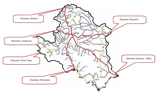
Fig. 1. Nowy
Sącz district – most dangerous routes
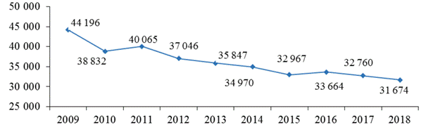
Fig. 2. Road accidents
occurrence trend from 2009 to 2018 year [7]
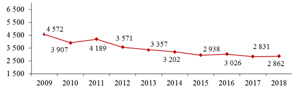
Fig. 3. Road accidents fatal
casualties trend from 2009 to 2018 year [7]
To
secure accident casualties against damage, the Act of 2 December 1958 on
property and personal insurance (Journal of Laws No. 72, item 357, Art. 5, as
amended) introduced two types of compulsory insurance:
·
civil liability insurance of owners and drivers of motor vehicles
against damage caused in traffic,
·
insurance against all accidents to passengers or other casualties in
motor vehicle traffic.
Over
the years, compulsory vehicle insurance rules have been updated and revised.
Currently, it is governed by the Act of 22 May 2003 on compulsory insurance,
the Insurance Guarantee Fund and Polish Motor Insurers' Bureau. According to
Art. 23 thereof, the owner of a motor vehicle is obliged to sign a compulsory
liability insurance agreement covering damage caused in relation to
participation in traffic.
Damage
occurs as a consequence of random events. The general legal definition of
“damage” says that it consists of a breach of legally protected
property and interest, which can only be repaired if other liability
requirements are fulfilled. Additionally, damage entails any material or
non-material losses.
In
the analysed period, the insurance company participating in the study
registered 15,458 damage cases.
3. GREY SYSTEM THEORY
The
Grey System Theory was developed in the early 1980s. The concept refers to an
operational condition of an item, in which a certain amount (part) of data
describing a given parameter is known (that is, is clearly defined), while the
other part is unknown. The “Grey System Theory” method uses the
known part of information to determine (predict) the unknown part. The
character of the system is controlled in advance to shape its future
development. The Grey System Theory is used in forecasting events in
economics and agriculture. It was originally used for machine health monitoring
and troubleshooting. This prediction theory works mainly with past data to
create a mathematical model simulating time cycle data. If the required
measurement accuracy cannot be obtained, it is compensated and rectified by
identifying the “remaining data” until proper prediction results
are reached.
The
Grey System Theory has been applied in many fields of science and life. Wang et
al. (2020), used this method to predict the municipal demand for heat
production [8]. The authors of [9] predicted highway traffic intensity, while authors
of [10] dealt with time series prediction applied to road traffic safety in
Germany. The Grey System Theory has been applied in the health care sector
[11], in surface engineering to predict pitting fatigue [12], and also in
logistics, to support freight delivery related decisions [13] or in prediction
of diagnostic symptom values [14].
The
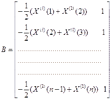
model of grey system is described with the following differential equation:
![]() (1)
(1)
Parameters
“a” and “u” can be calculated by determining the X1(k) model, previously
denoted as the sum of input values of X0(t) models for
i=l,2,...,k.
![]() (2)
(2)
The Grey System Model
derives from the obtained data. Then, the answer or predictive equation has the
following form:
![]() (3)
(3)
Parameters
“a” and “u” can be calculated using the following
equation:
![]()
according to the least
squares method:
![]() (4)
(4)
where B is the following
data matrix:
 (5)
(5)
![]() (6)
(6)
If
the required model accuracy cannot be reached, it is compensated and rectified
by identifying the “remaining data” of the model.
The
following data strings will be determined using Equation 3:
![]()
Predicted data are
calculated in the following way:
![]()
![]() (7)
(7)
The rest of the cycle is
calculated using the following equation:
![]() (8)
(8)
k=1,2,...,n
Having
calculated the rest of the cycle![]() ,
other predicted values can be obtained using Equation 3. Next, the values of
the remaining part of the prognosis should be added to the results of
prediction X(0)(k). This process can be repeated as many times as
required until model accuracy is reached.
,
other predicted values can be obtained using Equation 3. Next, the values of
the remaining part of the prognosis should be added to the results of
prediction X(0)(k). This process can be repeated as many times as
required until model accuracy is reached.
The
accuracy of the described method is determined using the following equation,
referred to as “remaining data”:
![]() (9)
(9)
where q(k) is the rest
of k data.
The
average value of real data X0(k) is denoted in the following form:
![]() , k=1,2,...,n (10)
, k=1,2,...,n (10)
The average value of the
“remaining data” q(k) is denoted in the following form:
![]() ,
, ![]() , k=1,2,...,n (11)
, k=1,2,...,n (11)
The variance of real
(measured) values S:
![]() (12)
(12)
The variance of the
“remaining data” S:
![]() (13)
(13)
The quotient of these
two values:
![]() (14)
(14)
is referred to as the
discrepancy quotient.
Calculated values C (Tab. 3) correspond to the lowest error probability
values P:
![]() (15)
(15)
which is equivalent to
classification of the prognosis in a proper accuracy group.
Tab. 3
Method accuracy prediction
|
Prognosis accuracy |
P |
C |
|
good |
>0.95 |
<0.35 |
|
satisfactory |
0.8-0.9 |
0.35-0.5 |
|
unsatisfactory |
0.7-0.8 |
0.5-0.65 |
|
poor |
<0.7 |
>0.65 |
In the analysed sample
predictions based on the “Grey System Theory”, predicted and actual
data (obtained in measurements) are quite consistent. The Grey System Theory
can be used in technical facilities condition inspections as one of the
monitoring system elements.
4. PREDICTING ECONOMIC INDICES IN VEHICLE INSURANCE
4.1. Presentation of processed data
As earlier mentioned in
the introduction section, the prognosis was prepared using statistical data
recorded by a certain insurance company operating in Poland, at the end of each
four-month settlement period in 2018 and 2019. Fig. 4 presents the insurance
economic indices included in the described prognosis.
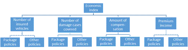
Fig. 4. Scheme
of predicted insurance economic indices
·
Package policies - provide comprehensive coverage of the vehicle and its
owner and include compulsory liability insurance, voluntary all-accident
insurance with Assistance insurance (technical support and medical aid in
Poland), post-accident coverage for driver and passengers. Offered to owners of
cars, vans and goods vehicles with gross vehicle weight up to 2 [t] in the
analysed insurance company.
·
Other policies - including all-accident insurance.
·
Number of insured vehicles - number of insurance agreements registered
in the analysed period.
·
Premium income - amount earned on the sale of insurance policies in the
analysed period.
·
Amount of compensation - amount of benefits paid in the analysed period.
·
Number of damage cases covered - number of damage cases compensated in
the analysed period.
Tab.
4 contains a summary of the input data needed by insurance companies for
qualitative and quantitative prediction of road accidents.
Tab.
4
Summary of input data
|
No. |
Period of analysis |
Number of insured vehicles |
Premium income [PLN] |
Number of damage cases
covered |
Amount of compensation
[PLN] |
|
Vehicles with package insurance
policies |
|||||
|
1 |
1st quarter of
2018 |
1,433 |
1.766,350 |
188 |
760,864 |
|
2 |
2nd quarter of
2018 |
1,729 |
2,104,945 |
170 |
678,343 |
|
3 |
3rd quarter of
2018 |
1,369 |
1,643,956 |
255 |
787,276 |
|
4 |
4th quarter of
2018 |
1.106 |
1,289,829 |
289 |
1,175,124 |
|
5 |
1st quarter of
2019 |
1,044 |
1,244,893 |
331 |
985,636 |
|
6 |
2nd quarter of
2019 |
1,019 |
1,292,606 |
260 |
878,857 |
|
7 |
3rd quarter of
2019 |
922 |
1,162,542 |
269 |
1,086,480 |
|
8 |
4th quarter of
2019 |
651 |
800,573 |
199 |
599,693 |
|
Vehicles with other
insurance policies |
|||||
|
1 |
1st quarter of
2018 |
1,130 |
1,047,601 |
274 |
1,225,717 |
|
2 |
2nd quarter of
2018 |
1,293 |
1,336,660 |
245 |
1,150,498 |
|
3 |
3rd quarter of
2018 |
1,095 |
1,117,935 |
199 |
915,445 |
|
4 |
4th quarter of
2018 |
1,144 |
1,049,565 |
178 |
813,200 |
|
5 |
1st quarter of
2019 |
1,362 |
1,375,988 |
214 |
1,216,293 |
|
6 |
2nd quarter of
2019 |
1,417 |
1,491,511 |
262 |
873,208 |
|
7 |
3rd quarter of
2019 |
1,356 |
1,432,006 |
289 |
1,441,465 |
|
8 |
4th quarter of
2019 |
9,095 |
10,235,056 |
267 |
1,134,300 |
4.2. Prognosis of economic indices of vehicle insurance
Tab.
5 contains a summary of input data divided into separate economic indices. Data
is presented in the descending order.
Tab.
5
Input data in descending order
|
|
I |
II |
III |
IV |
V |
VI |
VII |
VIII |
|
Number of damage cases covered –
package policies |
||||||||
|
|
331 |
289 |
269 |
260 |
255 |
199 |
188 |
170 |
|
Number of damage cases covered – other
policies |
||||||||
|
|
289 |
274 |
267 |
262 |
245 |
214 |
199 |
178 |
|
Amount of compensation – package
policies |
||||||||
|
|
117,5124 |
108,6480 |
985,636 |
878,857 |
787,276 |
760,864 |
67,8343 |
599,693 |
|
Amount of compensation – other
policies |
||||||||
|
|
144,1465 |
1,225,717 |
1,216,293 |
1,150,498 |
1,134,300 |
915,445 |
873,208 |
813,200 |
|
Premium income – package policies |
||||||||
|
|
2,104,945 |
1,766,350 |
1,643,956 |
129,606 |
1,289,829 |
1,244,893 |
1,162,542 |
800,573 |
|
Premium income – other policies |
||||||||
|
|
1,491,511 |
1,434,937 |
1,432,006 |
1,375,988 |
1,336,660 |
1,117,935 |
1,049,565 |
1,047,601 |
|
Number of insured vehicles – package
policies |
||||||||
|
|
1,729 |
1,433 |
1,369 |
1,106 |
1,044 |
1,019 |
922 |
651 |
|
Number of insured vehicles – other
policies |
||||||||
|
|
1,417 |
1,362 |
1,359 |
1,324 |
1,293 |
1,144 |
1,130 |
1,095 |
Using
the formulas presented in the previous section, prognosis equations for
individual economic indices was derived.
Number
of damage cases covered – package policies
![]()
Number of damage cases
covered – other policies
![]()
Amount of compensation
– package policies
![]()
Amount of compensation
– other policies
![]()
Premium income –
package policies
![]()
Premium income –
other policies
![]()
Number of vehicles
insured – package policies
![]()
Number of vehicles
insured – other policies
![]()
Tab.
6 contains a summary of input data and predicted values calculated using the
equations presented above. A – stands for input value, B –
predicted value. Figs. 5 to 8 present the distribution of analysed economic
indices of the insurance business.
Tab. 6
Summary of input data and predicted values
|
|
I |
II |
III |
IV |
V |
VI |
VII |
VIII |
IX |
X |
XI |
XII |
|
Number of damage cases covered –
package policies |
||||||||||||
|
A |
331 |
289 |
269 |
260 |
255 |
199 |
188 |
170 |
- |
- |
- |
- |
|
B |
331 |
298 |
273 |
250 |
229 |
210 |
192 |
176 |
162 |
148 |
136 |
125 |
|
Number of damage cases covered – other
policies |
||||||||||||
|
A |
289 |
274 |
267 |
262 |
245 |
214 |
199 |
178 |
- |
- |
- |
- |
|
B |
289 |
286 |
267 |
249 |
232 |
216 |
201 |
188 |
175 |
163 |
152 |
142 |
|
Amount of compensation – package
policies x 1000 |
||||||||||||
|
A |
1,175 |
1,086 |
985 |
878 |
787 |
760 |
678 |
599 |
- |
- |
- |
- |
|
B |
1,175 |
1,079 |
980 |
891 |
809 |
735 |
668 |
607 |
552 |
501 |
455 |
414 |
|
Amount of compensation – other
policies x 1000 |
||||||||||||
|
A |
1,441 |
1,225 |
1,216 |
1,150 |
1,134 |
915 |
873 |
813 |
- |
- |
- |
- |
|
B |
1,441 |
1,285 |
1,196 |
1,113 |
1,036 |
964 |
897 |
835 |
777 |
723 |
672 |
626 |
|
Premium income – package policies x
100 |
||||||||||||
|
A |
21,049 |
17,663 |
16,439 |
12,926 |
12,898 |
12,448 |
11,625 |
8,005 |
- |
- |
- |
- |
|
B |
21,049 |
17,647 |
15,877 |
14,284 |
12,851 |
11,562 |
10,403 |
9,359 |
8,420 |
7,576 |
6,816 |
6,132 |
|
Premium income – other policies x 100 |
||||||||||||
|
A |
14,915 |
14,349 |
14,320 |
13,759 |
13,366 |
11,179 |
10,495 |
10,476 |
- |
- |
- |
- |
|
B |
14,915 |
14,980 |
14,092 |
13,256 |
12,470 |
11,730 |
11,034 |
10,380 |
9,764 |
9,185 |
8,640 |
8,128 |
|
Number of insured vehicles – package
policies |
||||||||||||
|
A |
1,729 |
1,433 |
1,369 |
1,106 |
1,044 |
1,019 |
922 |
651 |
- |
- |
- |
- |
|
B |
1,729 |
1,459 |
1,309 |
1,174 |
1,052 |
944 |
846 |
759 |
681 |
610 |
547 |
491 |
|
Number of insured vehicles – other
policies |
||||||||||||
|
A |
1,417 |
1,362 |
1,359 |
1,324 |
1,293 |
1,144 |
1,130 |
1,095 |
- |
- |
- |
- |
|
B |
1,417 |
1,401 |
1,345 |
1,291 |
1,239 |
1,190 |
1,142 |
1,096 |
1,052 |
1,010 |
969 |
931 |
a) 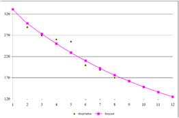 b)
b) 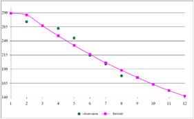
Fig. 5. Number of damage cases covered a) package
policies, b) other policies
a)  b)
b) 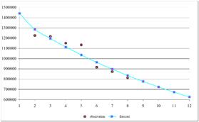
Fig. 6. Amount of paid compensation a) package
policies, b) other policies
a) 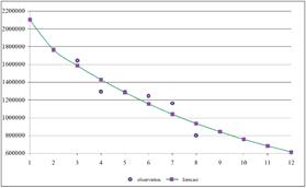 b)
b) 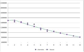
Fig. 7.
Premium income amount a) package policies, b) other policies
a) 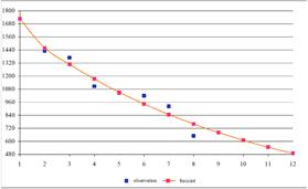 b)
b) 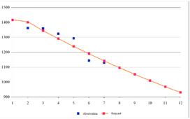
Fig. 8.
Number of insured vehicles a) package policies, b) other policies
The accuracy of the
method has been determined using Equations 10 to 13. Probability P for each ![]() exceeds 0.95 in all analysed indices.
This posits that the proposed method is correct.
exceeds 0.95 in all analysed indices.
This posits that the proposed method is correct.
5. CONCLUSIONS
The results presented in
Section 4 indicate that the prognosis suggested a probable decrease in the
value and quantity of each analysed economic index of vehicle insurance.
The decreasing trend is
reasonably related to the number of insurance policies and the amount of paid
compensation. The number of newly registered cars for which liability insurance
is legally required is constantly increasing. Road statistics with reference to
the number of cars cited in 2.3 above show a decreasing trend. The value of
paid compensation is largely affected by the post-accident repair cost
estimate. The number of used cars imported to Poland is still high. Although
their age varies, most cars are several years old. Costs of accident repairs in
these vehicles quite often exceed their market value, which is reflected in
lower amounts of paid compensation.
Currently, monitoring of
the analysed indices is about to start so as to verify if the results obtained
using the Grey System Theory method correspond to the actual economic situation
in 2020.
References
1.
Bodziony
M., T. Kądziołka, A. Kochanek, S. Kowalski. 2016. “Work time analysis of drivers in the aspect of
road traffic safety”. Autobusy:
technika, eksploatacja, systemy transportowe 6: 85-94. ISSN 1509-5878.
2.
Kądziołka
T., S. Kowalski. 2016. “Analysis of road traffic safety exemplified by
selected road crossings”. Autobusy:
technika, eksploatacja, systemy transportowe 12: 235-241. ISSN 1509-5878.
3.
Kowalski S., A.
Zwolenik. 2019. “Analysis of the company's operating costs on the example
of a transport company”. Autobusy:
technika, eksploatacja, systemy transportowe 6: 311-314. ISSN 1509-5878.
4.
Bodziony
M., T. Kądziołka, A. Kochanek, S. Kowalski. 2016. “Work time analysis of drivers in the aspect of
road traffic safety”. Autobusy:
technika, eksploatacja, systemy transportowe 6: 85-94. ISSN 1509-5878.
5.
Kądziołka
T., A. Kochanek, S. Kowalski, 2016. “Cost
analysis of fuel consumption by motor vehicles”. Prace Naukowe Politechniki Warszawskiej. Transport 112: 175-183.
ISSN 1230-9265.
6.
Wyborkierowcow.pl.
“The
worst and best insurance companies in 2019”. Available at: https://www.wyborkierowcow.pl/najgorsze-i-najlepsze-firmy-ubezpieczeniowe-w-2019-roku/.
7.
„Knowledge
base - Statistics”. Available at: https://www.krbrd.gov.pl/.
8.
Wang S., P. Wang,
Y. Zhang. 2020. “A prediction method for urban heat supply based on grey
system theory”. Sustainable Cities
and Society 52: 1-7.
9.
Anton Bezuglov A.,
G. Comert. 2016. “Short-term
freeway traffic parameter prediction: Application of grey system theory models”.
Expert Systems with Applications 62: 284-292.
10.
Hosse René
S., U. Becker, H. Manz. 2016. “Grey systems theory time series prediction
applied to road traffic safety in Germany”. IFAC-PapersOnLine
49(3): 231-236.
11.
Jui-Chen Huang.
2011. “Application
of grey system theory in telecare”. Computers in
Biology and Medicine 41: 302-306.
12.
Ma F.Y., W.H.
Wang. “Prediction of
pitting corrosion behavior for stainless SUS 630 based on grey system theory”.
Materials
Letters 61: 998-1000.
13.
Alfaro-Saiz J.J.,
M.C. Bas, V.G. Bosch, R. Rodríguez-Rodríguez, M.J. Verdecho.
“An evaluation
of the environmental factors for supply chain strategy decisions using grey systems
and composite indicators”. Applied
Mathematical Modelling: 1-16
14.
Tabaszewski M.
2014. “Prediction of diagnostic symptom values using a set of models
GM(1,1) and a moving window method”. Diagnostyka
15(3): 65-68.
Received 02.03.2020; accepted in revised form 17.05.2020
![]()
Scientific
Journal of Silesian University of Technology. Series Transport is licensed
under a Creative Commons Attribution 4.0 International License