Article
citation information:
Dogan, E. Analysis and comparison of long
short-term memory networks short-term traffic prediction performance. Scientific Journal of Silesian University of
Technology. Series Transport. 2020, 107,
19-32. ISSN: 0209-3324. DOI: https://doi.org/10.20858/sjsutst.2020.107.2.
Erdem DOGAN[1]
ANALYSIS
AND COMPARISON OF LONG SHORT-TERM MEMORY NETWORKS SHORT-TERM TRAFFIC PREDICTION
PERFORMANCE
Summary. Long short-term memory networks (LSTM) produces
promising results in the prediction of traffic flows. However, LSTM needs large
numbers of data to produce satisfactory results. Therefore, the effect of LSTM
training set size on performance and optimum training set size for short-term
traffic flow prediction problems were investigated in this study. To achieve
this, the numbers of data in the training set was set between 480 and 2800, and
the prediction performance of the LSTMs trained using these adjusted training
sets was measured. In addition, LSTM prediction results were compared with
nonlinear autoregressive neural networks (NAR) trained using the same training
sets. Consequently, it was seen that the increase in LSTM's training cluster
size increased performance to a certain point. However, after this point, the
performance decreased. Three main results emerged in this study: First, the
optimum training set size for LSTM significantly improves the prediction
performance of the model. Second, LSTM makes short-term traffic forecasting
better than NAR. Third, LSTM predictions fluctuate less than the NAR model
following instant traffic flow changes.
Keywords: deep learning, traffic flow, short-term,
prediction, LSTM, nonlinear autoregressive, training set size
1. INTRODUCTION
Nowadays,
the number of vehicles and travel demands are increasing rapidly. This increase
is responsible for delays, fuel loss and high emissions globally. For this
reason, the efficiency of road capacities should be increased by directing and
controlling road traffic with intelligent transport systems (ITS). However, ITS
needs information about the current status of traffic variables and future
estimates of this information (for example, volume, speed, travel time, etc.).
For ITS to be more efficient, it is important that traffic parameters be
accurately estimated, especially in the short term. Thus, ITS can make fast and
accurate decisions for future traffic situations. For this reason, studies on
predicting the short-term future situation of traffic become important.
Researchers are working to make these predictions more accurate by developing
new methods. Especially as deep learning has proven itself in many areas, the
use of deep learning in short term traffic prediction has accelerated.
Therefore, there is a need for research that better demonstrates the potentials
of deep learning in this regard.
The first
study on short-term traffic flow estimation was performed using the Box-Jenkins
method [1]. Time
series methods were used to estimate traffic flow in other studies. [2-8] However,
when artificial intelligence approaches and time series methods were compared,
it was observed that artificial intelligence predicted short term traffic flow
better [9]. Therefore,
in this study, traffic flow estimation models were developed by using
artificial intelligence and deep networks approaches and the size of the
training sets were discussed [10].
Short-term traffic flow estimation was performed with ANNs in earlier times
from deep learning approach. For instance, the dynamic wavelet ANN model was
used to estimate traffic flow [11]. Dynamic
traffic flow modelling is another approach to determine the amount of traffic
flow [12]. ANN and K-NN
were used together to estimate traffic flow [13]. In another
study, multiscale analysis-based intelligent ensemble modelling was used to
predict airway traffic [14]. The
traffic flow was modelled for the city of Istanbul using different time
resolutions and the results were accurate despite the limited data [15] and some
others [15-18]. Deep
learning has recently gained interest in the prediction of various traffic
parameters. Long short-term memory (LSTM) is in the sub-branch of deep
learning. Previous studies on LSTM have evidence that deep learning and the
performance of other methods were compared. For example, LSTM was compared with
regression models [19]. As a
result, LSTM has generally made better predictions, except in some cases. Researchers
developed a model using LSTM to predict the short-term traffic flow in
exceptional traffic conditions. In addition, the authors studied the
characteristics of traffic data [20]. In another
study, LSTM and recurrent ANN models were compared with ARIMA models [21]. As a
result, researchers mentioned that artificial intelligence models work better.
In the other study, LSTM and recurrent ANN and regression models were compared
with LSTM obtaining better results [22].
LSTM and
short-term traffic flow were reviewed in the literature, but so far, there was
no study on the effect of training set size on LSTM performance. Therefore, in this study, LSTM and
nonlinear autoregressive neural networks (NAR) were trained with different
training sets size and the optimum size was determined for the problem. In
addition, two models were compared, and their results discussed. Thus, the
results of this study will help to determine the size of the training set for
future studies.
This article
consists of introduction, methodology and conclusion. The subject and
importance of this study are discussed, and the related literature is
summarised in the introduction section of this article. The data used and
the estimation of missing data are presented in the methodology section. Then,
LSTM and NAR approaches were briefly explained, and the parameters of the
models used in the study were introduced. Thereafter, NAR and LSTM estimates
were tested by hypothesis testing and the results were discussed. Finally, the
conclusions of the study were recalled in the conclusion section and
recommendations were made for future studies.
1. METHODOLOGY
1.1. Data collection
and missing data
Traffic flow data were collected
from the D200 highway. This highway connects the major cities of Turkey. The
main road traffic is not interrupted 20 km forward and backward from the
counted section. Therefore, there are uninterrupted conditions in the counting
section. Data collection was performed with NC-350 traffic counters [23]. The counting was conducted with
traffic counting devices placed separately for the left and right lanes. The
devices were set to record data every 15 minutes. Devices were counted for 47
days and 4,512 traffic flow data were collected.
In the counting process, data cannot
be recorded at some time intervals and this is very common. This data is called
missing data. This is often the result of faults in the device or the
limitations of the counting device. After counting operations, it was found
that approximately 1% of the total data was missing. Autocorrelation reveals
the degree of relationship of time series points with each other. The points
with high autocorrelation are used in making future predictions. To complete
the missing data, traffic data with high autocorrelation were used with missing
data. The results of the autocorrelation calculation result are given in Fig.
1. Autocorrelation was high at point 672. Each counting operation has 15 min
intervals. In other words, every point in the time series is related to the
point 7 days (672 / (24 * 4) previous. This is a very common pattern in traffic
flows.
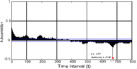
Fig. 1. Completion of missing data
In this
case, the missing data can be completed with the value at the point 672
interval before the missing point. Let X ∊ ℤ be traffic data with missing values and xt ∊ X indicates
the traffic flow data at time t. Also, let ![]() ∊ ℤ denote the
missing data in the series and at time t.
According to these definitions, the missing data is completed as in Equation 1.
∊ ℤ denote the
missing data in the series and at time t.
According to these definitions, the missing data is completed as in Equation 1.
![]() (1)
(1)
After
completing the missing data, the data set was standardised with Equation 2
before training the models.
![]() (2)
(2)
where,
xstd standardised
data,
x raw
data,
![]() mean
of the dataset,
mean
of the dataset,
sx standard
deviation of the dataset.
1.2.
Long short-term memory
Long
short-term memory network (LSTM) is an advanced type of recurrent neural
networks (RNNs) that can overcome the long-term dependence problem. RNNs
produced successful results in sequence prediction tasks. However, it is often
difficult for RNNs to learn long-term patterns [24]. LSTM can
understand short- or long-term dependencies with the help of units that learn
when to forget and when to update the information.
Let xt be
the input vector, ht be the output of the LSTM unit and Ct be the cell
state at time t. In the first step, how much of the
information in the Ct-1
will be forgotten is determined by forget gate.
The forget gate is a layer that uses sigmoid function and uses ht-1
and xt to generate
values between “0” and “1”. Therefore, ft in Fig. 2 can be written
as:
![]() (3)
(3)
The next
step is to identify new information that will be stored in the cell state. This
step consists of two sub-steps: The first step is the input gate, which determines what information to update. The second
step determines the vector containing the candidate values. In Fig. 2, the
output value of the input gate is
represented by it, while
the output value of the second section is indicated by ![]() . The it and
. The it and ![]() can be written as:
can be written as:
![]() and
and ![]() (4)
(4)
After these
steps, the old state vector (Ct-1) is updated to reveal the new state vector (Ct). The update process can be written
as:
![]() (5)
(5)
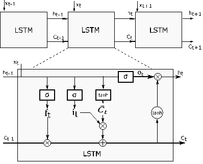
Fig. 2. Long
short-term memory network unit
The last step is to
determine the hidden state (ht):
![]() (6)
(6)
The output
gate (ot)
is the process that determines which parts of the cell state will be in the
output and can be written as:
![]() (7)
(7)
where σ() is the sigmoid function, W(f,i,c,o)
matrices are the network parameters, b(f,i,c,o) is the bias matrices. And ⊙ denotes the
product operation. LSTM can successfully overcome the exploding/vanishing
gradients problem with these processes and gates [25].
1.3.
Nonlinear
auto-regressive neural networks
Nonlinear autoregressive neural
networks (NAR) are a customised neural network (ANN) model for time series. NAR
predicts the future value by using the past data of the time series. NAR needs
a training set like other ANNs. Let X ∊ ℤ be the traffic flow data and xt ∊ X denotes the traffic flow value at time t. In this case, the future
traffic flow value will be: x ̂_(t+1)=f(x_t,x_(t-1),…x_(t-d)).
Where, x ̂_(t+1) is the prediction value of the NAR, f(x) expresses the
NAR black-box function and the d is the delay value. Backpropagation algorithm [26] and Levenberg-Marquardt method [28,29] were used for training.
The connections of the NAR with the
hidden and the output layers are shown in Fig. 3. The model uses a delay
parameter ![]() to estimate the traffic flow
to estimate the traffic flow ![]() at time t + 1. In this study, in the hidden layer tangent hyperbolic and in
the output layer linear function were used as activation functions. To
determine the appropriate NAR architecture, the number of hidden layer neurons
was tested from 5 to 35. Then, the RMSE of different NAR architectures were
analysed and it was decided that 3-10-1 was the appropriate NAR architecture.
at time t + 1. In this study, in the hidden layer tangent hyperbolic and in
the output layer linear function were used as activation functions. To
determine the appropriate NAR architecture, the number of hidden layer neurons
was tested from 5 to 35. Then, the RMSE of different NAR architectures were
analysed and it was decided that 3-10-1 was the appropriate NAR architecture.
In this section, we first introduced
the creation of training and test sets. Then, the effect of the size of the
training sets on the predictions of NAR and LSTM was examined and finally, the
prediction results of the two methods were evaluated by statistical tests.

Fig. 3. Nonlinear autoregressive neural
network architecture
Traffic flow vector (X) consists of 47 daily traffic flow
data. The data sets to be used for training were selected in six different
sizes from 5 to 30 days. Let ej
⊂ X be a training set vector and the number of data
in ej will be ![]() and j=1,2,…,6.
The last 17 days of the X vector
were selected for testing the models. Let tm
⊂ X be a test set vector and m=1,2,…,17.
and j=1,2,…,6.
The last 17 days of the X vector
were selected for testing the models. Let tm
⊂ X be a test set vector and m=1,2,…,17.
The pseudo-code for the creation of
training and test sets with these representations is as follows:
1. Start
2. Let, n := |X|, r :=|tm|, p :=|ej|,
3. m = 1,
4. j = 1,
5. ej = {xt | (t>(n-(j*r+p) ⋀ t≤(n-j*R)}
6. tm={{xt | (t>(n-(j*r) ⋀ t≤(n-(( j-1)*r)),
7. If j < p and m<r Then,
j = j + 1 and turn back to Step 4
If j = p and m<r Then,
m= m + 1 and turn back to Step 4
If j = p and m = r Then, Stop.
The delay
parameter ![]() or lag value was kept equal in the LSTM
and NAR models, and this value was set to
or lag value was kept equal in the LSTM
and NAR models, and this value was set to![]() . Thus, regardless of parameter d, the effect of data set size on
performance was compared.
. Thus, regardless of parameter d, the effect of data set size on
performance was compared.
NAR and LSTM models with training
set size 480 ![]() were named NAR5 and LSTM5 and the test
results were given in Fig. 4 using box-plot. In Figs. 4 and 5, the outliers
were shown with the (+) sign. If these (+) signs are
counted from Figs. 4 and 5, it is understood that while LSTM produces ten
outliers, the NAR has four outliers. This result indicates that LSTM predictions
are rarely more than expected. When
the median values were examined, it was seen that the value of NAR5 was higher
than the value of LSTM5. In addition, it was observed that the range of LSTM5
was smaller than NAR5 with the examination of the upper/lower whiskers. Simply
put, the LSTM approach was able to produce better results than the NAR with the
smallest training set size examined.
were named NAR5 and LSTM5 and the test
results were given in Fig. 4 using box-plot. In Figs. 4 and 5, the outliers
were shown with the (+) sign. If these (+) signs are
counted from Figs. 4 and 5, it is understood that while LSTM produces ten
outliers, the NAR has four outliers. This result indicates that LSTM predictions
are rarely more than expected. When
the median values were examined, it was seen that the value of NAR5 was higher
than the value of LSTM5. In addition, it was observed that the range of LSTM5
was smaller than NAR5 with the examination of the upper/lower whiskers. Simply
put, the LSTM approach was able to produce better results than the NAR with the
smallest training set size examined.
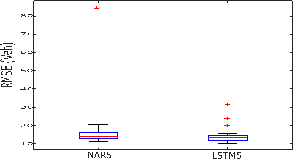
Fig. 4.
Comparison of errors for trained models with different-sized training sets
Fig. 5 shows the RMSE values
produced by the models as a result of the use of training set sizes between 10
and 30 days. It can be read from the median lines depicted in Fig. 5 that the
LSTM produces lower RMSE for all training set sizes. It was observed that NAR
error values were oscillated by increasing the size of the training set, but no
clear decrease was observed. Furthermore, it is understood from Fig. 5 that the
LSTM error values tend to decrease clearly for the same training set size
increase. Thus, following examination of the average RMSE values of the models,
it was found that the lowest error was in ![]() for NAR and LSTM. Based on this, the
error values of the models due to their training with
for NAR and LSTM. Based on this, the
error values of the models due to their training with ![]() , training set size were examined
more closely. Fig. 5 shows that the maximum RMSE value of NAR25 is 17 veh.
However, the maximum prediction error value of LSTM25 was about 13 veh.
, training set size were examined
more closely. Fig. 5 shows that the maximum RMSE value of NAR25 is 17 veh.
However, the maximum prediction error value of LSTM25 was about 13 veh.
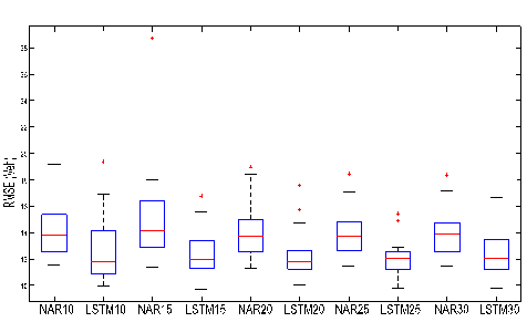
Fig. 5. Comparison of errors
for trained models with different-sized training sets
To observe the prediction of the
models in more detail, the 17th test day was examined in Fig. 6. And to observe
the estimations of the models in more detail, the 17th test day was examined in
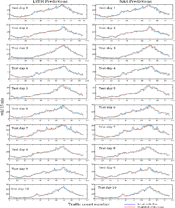
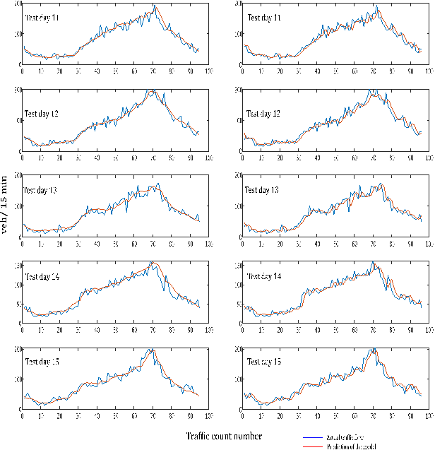
Fig. 6. The results of the remaining test days are presented in Appendix 1 for
the reader's review. The coefficients of estimation of the two models were
calculated and it was determined that both models produced high R2
values. The calculated R2 values for the remaining days can be
examined in Appx 2 and 3. Like the RMSE values examined in the previous figures,
LSTM predictions produced R2 values higher than NAR predictions for
all test days. A remarkable situation was seen during the comparison of the
models on the line graph. In Fig. 6, the prediction line of NAR makes high
fluctuations to approach the actual value. On the other hand, the fluctuation
of LSTM was less than NAR. The same examination was performed for the other
test days and the same result was reached. In the light of these results, it
was concluded that LSTM was less affected by instant traffic flow changes than
NAR model.
Although the LSTM was found to be
more accurate than NAR, the statistical significance of this result was tested
by t-test. The established hypothesis statements were established as follows:
H0: If LSTM is used instead of NAR, the mean RMSE does not change. (μLSTM =μNAR)
H1: If LSTM is used instead of NAR, the mean RMSE is decreased. (μNAR> μLSTM)
where, μNAR and μLSTM
represent the mean of the estimation errors of NAR and LSTM,
respectively.
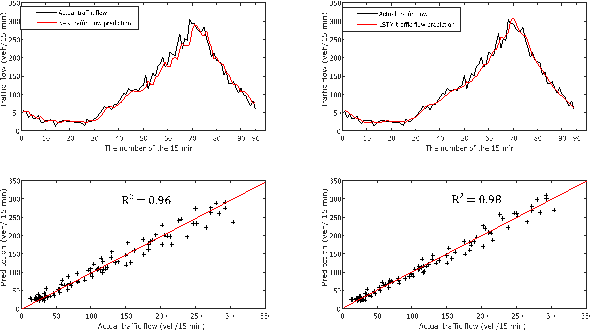
Fig. 6. Comparison of NAR25 and LSTM25 short-term traffic flow predictions with real values. (t-1) of the 15 min
The results of the paired t-test are summarised
in Tab. 1. Tab. 1 shows that the mean difference values (μ) of the two
models are positive for all ej's.
This indicates that the LSTM as less mean prediction errors than NAR. The
confidence level of the hypothesis test was 95% (α = 0.05). The p-value was examined from the table and it was
seen that p <0.05 was found for
the other training set sizes except for the 5-day training set. In the light of
these results, except for 5-day training set, H0 was rejected and H1
was accepted.
Paired t-test results (α =
0.05)
|
Number of data/ Number of days |ej| |
μ |
σ |
σx̅ |
Lower |
Upper |
t |
df |
p-value |
Result |
|
480 / 5 days |
4,21 |
13,48 |
3,27 |
-2,73 |
11,14 |
1,29 |
16 |
0,217 |
Ho Accept |
|
960 / 10 days |
1,46 |
0,70 |
0,17 |
1,10 |
1,82 |
8,56 |
16 |
0,000 |
Ho Reject |
|
1440 / 15 days |
2,71 |
4,38 |
1,06 |
0,46 |
4,97 |
2,55 |
16 |
0,021 |
Ho Reject |
|
1920 / 20 days |
1,74 |
1,05 |
0,25 |
1,20 |
2,28 |
6,85 |
16 |
0,000 |
Ho Reject |
|
2400 / 25 days |
1,73 |
1,01 |
0,24 |
1,21 |
2,25 |
7,08 |
16 |
0,000 |
Ho Reject |
|
2880 / 30 days |
1,58 |
0,73 |
0,18 |
1,20 |
1,95 |
8,92 |
16 |
0,000 |
Ho Reject |
The statistical analysis confirmed
that the LSTM model usually predicted traffic flow more accurately than the NAR
model for 15-min data. In addition, the improvement in the predictive
performance of the NAR model was not observed by increasing the size of the
training set. However, the improvement in the predictive performance of the
LSTM model was clearly observed by increasing the size of the training set.
However, it was determined that the increase in the size of the training set
should be at certain levels. For this study, it was found that this size should
have 2400 data (25 days) number for both models.
3. CONCLUSION
Accurate short-term traffic
forecasts will improve the decision-making capabilities of traffic control
systems. Thus, traffic flow and traffic safety will reach better levels. In
this study, training sets of different sizes were created. Then, the effects of
these clusters on the predictive performance of LSTM and NAR models were
examined. In terms of short-term traffic estimation, it was understood from the
analysis results and statistical tests that LSTM models have better predictions
than NAR models.
The conclusions of this study are as follows:
· This study showed that a large amount of training set
does not increase performance. For this reason, the optimum training set size
of the new deep learning approaches should be determined.
· The larger training set size does not always mean
better performance for LSTM and NAR.
· Improvement in LSTM estimation performance is observed
towards optimum training set size. However, the same feature cannot be
mentioned for NAR.
· LSTM is less affected by instant traffic flow changes
than the NAR model. Therefore, LSTM produces stable results from NAR for
short-term traffic prediction.
· Statistically, the LSTM approach performs better than
that of NAR when the training set size is greater than 480.
· It was observed that LSTM produced more outliers than
NAR. Therefore, in rare cases, LSTM is likely to make high errors.
· In this study, the size of the LSTM training set was
discussed in the context of the prediction of traffic flow. The effects of
other parameters of LSTM will be investigated in future studies. For this
study, tests were performed for a time interval of 15 minutes, which is
commonly used in the literature. In addition, smaller time intervals can be
investigated in future studies. Another limitation of this study is the use of
only one data set. Future studies will be enriched with different data sets
from different regions.
ITS will be an indispensable tool in the future
traffic control of cities. This will make future traffic flow forecasts much
more important. Therefore, it can easily be foreseen that the studies will
continue for more effective use of deep learning in road traffic prediction.
References
1.
Ahmed M.S., A.R.
Cook. 1979. „Analysis of freeway traffic time-series data by using
box-jenkins techniques”. Transportation Research Record. DOI:
https://doi.org/10.3141/2024-03.
2.
Çetiner
B., M. Sari, Borat O. 2010. „A neural network based traffic-flow
prediction model”. Mathematical and Computational Applications 15(2): 269-278.
3.
Chen C., J. Hu,
Q. Meng, Y. Zhang. 2011. „Short-time traffic flow prediction with
ARIMA-GARCH model”. IEEE Intelligent Vehicles Symposium. Proceedings
100084(Iv): 607-612. DOI:
https://doi.org/10.1109/IVS.2011.5940418.
4.
Dai X., R. Fu, Y.
Lin, L. Li, F.-Y. Wang. 2017. „Deeptrend: A deep hierarchical neural
network for traffic flow prediction”. ArXiv Preprint ArXiv 1707.03213.
5.
Doğan E.
2018. „Developing short-term traffic forecasting models using seasonal
ARIMA method for D-200 highway”. Sakarya University Journal of Science
22(2): 1-1. DOI:
https://doi.org/10.16984/saufenbilder.308997.
6.
Doğan E.
2020. „Short-term traffic flow prediction using artificial intelligence
with periodic clustering and elected set”. Promet-Traffic&Transportation
32(1): 65-78.
7.
Dunne S., B.
Ghosh. 2012. „Regime-based short-term multivariate traffic condition
forecasting algorithm”. Journal of Transportation Engineering 138: 455-466. DOI:
https://doi.org/10.1061/(ASCE)TE.1943-5436.0000337.
8.
Fu R., Z. Zhang,
L. Li. 2016. „Using LSTM and GRU neural network methods for traffic flow
prediction”. 31st Youth Academic Annual Conference of Chinese
Association of Automation (YAC):
324-328. IEEE.
9.
Fulari S., A.
Thankappan, L. Vanajakshi, S. Subramanian. 2019. „Traffic flow estimation
at error prone locations using dynamic traffic flow modeling”. Transportation
Letters 11(1): 43-53. DOI:
https://doi.org/10.1080/19427867.2016.1271761.
10. Hecht-Nielsen R. 1992. „Theory of the
Backpropagation Neural Network”. Proceedings
of the International Joint Conference on Neural Networks 1: 593-611. June
1989. IEEE. Academic Press. DOI:
https://doi.org/https://doi.org/10.1016/B978-0-12-741252-8.50010-8.
11. Hochreiter S. 1998. „The vanishing gradient
problem during learning recurrent neural nets and problem solutions”. International
Journal of Uncertainty, Fuzziness and Knowledge-Based Systems 6(02): 107-116.
12. Jiang X., H. Adeli, H.M. Asce. 2005. „Dynamic
wavelet neural network model for traffic flow forecasting”. Journal of
Transportation Engineering 131(10):
771-779. DOI: https://doi.org/10.1061/(ASCE)0733-947X(2005)131:10(771).
13. Kumar K., M. Parida, V.K. Katiyar. 2015. „Short
term traffic flow prediction in heterogeneous condition using artificial neural
network”. Transport 30(4):
397-405.
14. Levenberg K. 1944. „A method for the solution of
certain non-linear problems in least squares”. Quarterly Journal of
Applied Mathematics 2(2):
164-168. DOI: https://doi.org/10.1017/CBO9781107415324.004.
15. Lin S.-L.L.S.-L., H.-Q.H.H.-Q. Huang, D.-Q.Z.D.-Q.
Zhu, T.-Z.W.T.-Z. Wang. 2009. „The application of space-time ARIMA model
on traffic flow forecasting”. International Conference on Machine
Learning and Cybernetics 6:
12-15. DOI: https://doi.org/10.1109/ICMLC.2009.5212785.
16. Marquardt D.W. 1963. „An algorithm for
least-squares estimation of nonlinear parameters”. Journal of the
Society for Industrial and Applied Mathematics 11(2): 431-441. DOI: https://doi.org/10.1137/0111030.
17. Mccorbin Web Site. (n.d.). Available at:
http://www.mhcorbin.com/portable-traffic-analyzer/.
18. Polson N.G., V.O. Sokolov. 2017. „Deep learning
for short-term traffic flow prediction”. Transportation Research Part
C: Emerging Technologies 79:
1-17. DOI: https://doi.org/10.1016/j.trc.2017.02.024.
19. Shekhar S., B.M. Williams. 2008. „Adaptive
seasonal time series models for forecasting short-term traffic flow”. Transportation
Research Record: Journal of the Transportation Research Board 2024(1): 116-125. DOI:
https://doi.org/10.3141/2024-14.
20. Sheu J.-B., L.W. Lan, Y.-S. Huang 2009.
„Short-term prediction of traffic dynamics with real-time recurrent
learning algorithms”. Transportmetrica 5(1): 59-83. DOI: https://doi.org/10.1080/18128600802591681.
21. Tian Y., K. Zhang, J. Li, X. Lin, B. Yang. 2018.
„LSTM-based traffic flow prediction with missing data”. Neurocomputing
318: 297-305. DOI:
https://doi.org/https://doi.org/10.1016/j.neucom.2018.08.067.
22. Van Lint J.W.C., C. Van Hinsbergen. 2012.
„Short-term traffic and travel time prediction models”. Artificial
Intelligence Applications to Critical Transportation Issues 22: 22-41.
23. Williams B.M., L. Hoel. 2003. „Modeling and
Forecasting vehicular traffic flow as a seasonal ARIMA process: theoretical
basis and empirical results”. Journal of Transportation Engineering
129(6): 664-672. DOI:
https://doi.org/10.1061/(ASCE)0733-947X(2003)129:6(664).
24. Xiao Y., J.J. Liu, J. Xiao, Y. Hu, H. Bu, S. Wang,
2015. „Application of multiscale analysis-based intelligent ensemble
modeling on airport traffic forecast”. Transportation Letters 7(2): 73-79.
25. Yu R., Y. Li, C. Shahabi, U. Demiryurek, Y. Liu. 2017.
„Deep learning: a generic approach for extreme condition traffic
forecasting”. Proceedings of the 2017 SIAM International Conference on
Data Mining: 777-785. SIAM.
26. Zargari S.A., S.Z. Siabil, A.H. Alavi, A.H. Gandomi.
2010. „A computational intelligence-based approach for short-term traffic
flow prediction”. Expert Systems 29(2). DOI: https://doi.org/10.1111/j.1468-0394.2010.00567.x.
27. Zeng D., J. Xu, J. Gu, L. Liu, G. Xu. 2008.
„Short term traffic flow prediction using hybrid ARIMA and ANN
models”. Proceedings 2008 Workshop on Power Electronics and
Intelligent Transportation System. PEITS 2008. DOI:
https://doi.org/10.1109/PEITS.2008.135.
28. Zhou B., D. He, Z. Sun. 2006. „Traffic
predictability based on ARIMA/GARCH model”. 2nd Conference on Next
Generation Internet Design and Engineering, NGI 2006: 200-207. DOI: https://doi.org/10.1109/NGI.2006.1678242.
Appendix 1. Comparison of LSTM and NAR models
with actual values
Appendix 1
(contd). Comparison of LSTM and NAR models
with actual values
Received 02.04.2020; accepted in revised form 29.05.2020
![]()
Scientific
Journal of Silesian University of Technology. Series Transport is licensed
under a Creative Commons Attribution 4.0 International License