Article
citation information:
Bănică, M.V.,
Rădoi, A., Pârvu,
P.V. Onboard visual
tracking for UAV’s. Scientific Journal of Silesian
University of Technology. Series Transport. 2019, 105, 35-48. ISSN: 0209-3324. DOI: https://doi.org/10.20858/sjsutst.2019.105.4.
Marian Valentin BĂNICĂ[1],
Anamaria RĂDOI[2], Petrișor Valentin
PÂRVU[3]
ONBOARD VISUAL
TRACKING FOR UAV’S
Summary. Target tracking is one of the most common research
themes in Computer vision. Ideally, a tracking algorithm will only once receive
information about the target to be tracked and will be fast enough to identify
the target in the remaining frames, including when its location changes
substantially from one frame to another. In addition, if the target disappears
from the area of interest, the algorithm should be able to re-identify the
desired target. Target tracking was done using a drone with a Jetson TX2 computer onboard. The program
runs at the drone level without the need for data processing on another device.
Cameras were attached to the drones using a gimbal that maintains a fixed
shooting angle. Target tracking was accomplished by placing it in the centre of
the image with the drone constantly adjusting to keep the target properly
framed. To start tracking, a human operator must fit the target he wishes to
follow in a frame. The functionality of this system is excellent for remote
monitoring of targets.
Keywords: UAV, computer vision,
tracking
1. INTRODUCTION
The use of unmanned aircraft
technology and search, rescue and surveillance sensors is not a new idea. We
need to consider the number of operators required for a UAV system, a pilot to
control, plan and monitor the drones and a co-pilot to operate the sensors and
the flow of information. Because a man can focus on a limited number of tasks,
a computerised system, which optimises
the presentation of information and automates the data acquisition, is
necessary.
To automate the acquisition of
information suggests an attempt at integration of automatic video detection
systems for people, cars, and ships. Data produced in areas affected by a
disaster are georeferenced to support the presentation of information and
humanitarian action. Using the coordinates of the place where a photo
containing a target was done, the flight height and the position of the target
in the picture, the coordinates of the target can be calculated.
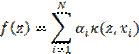
The primary goal of target tracking
is to determine the position of a selected target in a video. Based on the
initial state of a target in the first frame, the target-tracking algorithm
estimates the target position in subsequent frames. Many researchers have been
studying the issue of targeting for years and have come up with many solutions.
Nowadays, the main challenge comes from variations in lighting, occlusions, deformations,
rotations, and so on.
2. METHODOLOGY
The Moving Target
Indicator (MTI) is essential when the operator enlarges the area of interest to
observe details during a target tracking operation. If the area is greatly
enlarged, the operator will lose the overall image. This is often the case in
monitoring missions where the operator must detect the moving object, then recognise it (for example, an area where the movement
should be monitored). If more objects are moving, then all of them are detected
by identifying the motion of the pixel group. With this information, the
operator can focus his attention on the overall image and, if necessary, can
enlarge the image to extract more information about the object. In addition,
the operator can see all the moving objects, identify the direction of
movement, the set of moving objects and make the necessary decisions. The
motion detection part of the moving objects is the MTI tool's task.
In tracking, our goal is
to find a target in the current frame that we have successfully tracked in
previous frames. Based on the location and velocity (speed + direction of
motion) of the target in the previous frames, it is possible to predict the new
location from the current motion model with fair accuracy. Using vision tracking
it is easy to know how the target looks in each of the previous frames, so an
appearance model that encodes how the target looks like can be built. This
appearance model can be used to search in a small neighbourhood
of the location predicted by the motion model to more accurately predict the
location of the target. A simple template can be used as an appearance model if
the target is straightforward and does not change much in its appearance and
look for that template. However, this simple approach is not applicable in real
use-case scenarios because the appearance of a target can change dramatically.
To tackle this problem, in many modern trackers, this appearance model is a
classifier that is trained in an online manner.
In the following sections,
a review of the available tracking algorithms will be expounded. Next, a
proposal of a more efficient, energy-saving, moving model for the UAV to
maintain the target in the camera FOV (Field of View)
is highlighted. Afterwards, the results obtained from simulations and actual
flights are presented and conclusions are drawn.
3. TRACKING ALGORITHMS BASED ON ADABOOST SELECTION OF FEATURES
One of the first tracking methods that can work in
real-time was developed by Grabnet et al., and
was based on a feature selection algorithm called ADABOOST,
a name that comes from Adaptive Boosting, the algorithm that the HAAR cascade-based face detector uses internally. This
classifier needs to be trained at runtime with positive and negative examples
of the target. The initial bounding box supplied by the user is taken as the
positive example for the target, and many image patches outside the bounding
box are treated as the negative samples. For a new frame, the classifier is run
on every patch about the previous location and the score of the classifier is
recorded. The new location of the target is the one where the score is maximum.
This is one more positive example for the classifier. As more frames come in,
the classifier is updated with the additional data.
The basic idea for the ADABOOST algorithm is to combine a series of
“weak” classifiers with different weights to achieve a
"strong" classifier. Generally, binary decision trees or Nearest Neighbours are chosen as "weak" classification
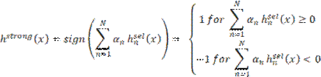
algorithms. Starting from M weak classifiers ![]() , a selector
, a selector ![]() will
select that “weak” classifier that minimises
a given cost function:
will
select that “weak” classifier that minimises
a given cost function:
|
|
(1) |
where ![]() is
the index of the minimum cost. The system consists of
is
the index of the minimum cost. The system consists of ![]() selectors. The selector's role is to
determine the best “poor” classifier for each extracted feature
type. Because of this, boosting algorithm is a feature selection algorithm.
selectors. The selector's role is to
determine the best “poor” classifier for each extracted feature
type. Because of this, boosting algorithm is a feature selection algorithm.
Thus, the result of a “strong” classifier for a
certain x patch is given by:
|
|
(2) |
where ![]() represents the class of the target being
tracked, and
represents the class of the target being
tracked, and ![]() represents the class corresponding to the
rest of the patches in the image and
represents the class corresponding to the
rest of the patches in the image and ![]() is
the weight associated with the nth selector and is calculated using
the formula:
is
the weight associated with the nth selector and is calculated using
the formula:
|
|
(3) |
where ![]() being the cost of the selector
being the cost of the selector ![]() .
.
4. TRACKING ALGORITHMS BASED ON MULTIPLE
INSTANCE LEARNING (MIL)
The MIL tracker has a similar approach when compared to the
ADABOOST tracker described above. The main difference
is that instead of considering only the current location of the target as a
positive example, it looks in a small neighbourhood
around the current location to generate several potential positive examples.
Tracking targets using the MIL technique has three main
components: representation of the image, classification model, and motion model
(2).
The classification model calculates the probabilities ![]() and
and ![]() where
where ![]() and
and ![]() represents the presence or absence of the
target from the analysed patch.
represents the presence or absence of the
target from the analysed patch. ![]() is the vector of traits extracted from the analysed patch. At each moment in time, the search of the
target is performed in the vicinity of the target location determined in the
previous frame, which allows the creation of a motion model. Thus, the patches
in the immediate vicinity of the previous location will be marked as positive
examples, and those outside of the neighbourhood will
be marked as negative examples.
is the vector of traits extracted from the analysed patch. At each moment in time, the search of the
target is performed in the vicinity of the target location determined in the
previous frame, which allows the creation of a motion model. Thus, the patches
in the immediate vicinity of the previous location will be marked as positive
examples, and those outside of the neighbourhood will
be marked as negative examples.
Learning a classification model using the MIL technique
involves the existence of a training set of form ![]() where
where ![]() is a
subset of patches
is a
subset of patches ![]() , and
, and ![]() is
the value
is
the value ![]() attached to this subset. Label
attached to this subset. Label ![]() if
there is at least one patch in the subset
if
there is at least one patch in the subset ![]() considered as a positive example.
considered as a positive example.
Thus, learning the classification model is equivalent to
finding the parameters that maximise the following
cost function:
|
|
(4) |
In the above equation, it is considered:
|
|
(5) |
whereas conditional probabilities like ![]() are
given by:
are
given by:
|
|
(6) |
where ![]() is a
"strong" classifier formed using the ADABOOST
feature selection technique presented in the previous section.
is a
"strong" classifier formed using the ADABOOST
feature selection technique presented in the previous section.
As in the previous case,
the system is trained in real-time and the user is only required to mark the
object to be tracked on the first frame of the video.
5. TRACKING ALGORITHMS BASED ON CORRELATION
FILTERS AND KERNEL METHOD
This type of trackers is built on the ideas presented in
the previous two sections. This tracker utilises the
fact that the multiple positive samples used in the MIL tracker have large
overlapping regions. This overlapping data leads to some nice mathematical
properties that were exploited to make tracking faster and more accurate at the
same time. Kernelized Correlation Filtering (KCF) aims to learn models effectively without reducing the
number of examples (3). Additionally, the Fourier transform, which converts a
convolution operation between two signals into a multiplication of the Fourier
transforms corresponding to the signals is used.
The purpose is to find a function ![]() which minimises the mean square
error between
which minimises the mean square
error between ![]() and
patches values
and
patches values ![]() :
:
|
|
(7) |
The second term of the sum is used for regularisation
and over-fitting control. The solution to a problem like the one above is:
|
|
(8) |
where ![]() is a
matrix formed by the vectors
is a
matrix formed by the vectors ![]() , and
, and ![]() is
the identity matrix,
is
the identity matrix, ![]() is a
vector formed by the patch’s values
is a
vector formed by the patch’s values ![]() . If the elements are complex numbers,
. If the elements are complex numbers, ![]() is
calculated as:
is
calculated as:
|
|
(9) |
where ![]() is conjugated−transposed matrices
is conjugated−transposed matrices ![]() .
.
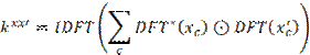
KCF takes into consideration that the training set may have
redundancy – a negative example, ![]() might be inserted into the dataset, along
with its cyclic permutations.
might be inserted into the dataset, along
with its cyclic permutations.
In matrix form, the patches and their circular permutations
can be written as
 , with
 ![]() being the generator element. Such a matrix
can be decomposed into:
being the generator element. Such a matrix
can be decomposed into:
|
|
(10) |
where: ![]() , with
, with ![]() and
and ![]() . Thus, the term
. Thus, the term ![]() of
equation (9) becomes:
of
equation (9) becomes:
|
|
(11) |
where ![]() is
the item-element multiplication operation.
is
the item-element multiplication operation.
But ![]() is
the autocorrelation in the frequency domain, also known as the spectral power
density.
is
the autocorrelation in the frequency domain, also known as the spectral power
density.
It is known
that for circular matrices, equation (9) is converted to:
|
|
(12) |
in which the fraction is calculated element-to-element.
Using the inverse discrete Fourier transform, the
parameters are obtained as ![]() .
.
A test patch ![]() is
evaluating using the function
is
evaluating using the function ![]() :
:
|
|
(13) |
To make the process more efficient, the authors propose
using the kernel method (3) that converts ![]() in:
in:
|
|
(14) |
in which ![]() are
patches from the training set,
are
patches from the training set, ![]() is
called kernel function and
is
called kernel function and ![]() is
the patch-like vector
is
the patch-like vector ![]() (for
example, raw pixels or HOG – Histogram of Oriented Gradients).
(for
example, raw pixels or HOG – Histogram of Oriented Gradients).
If the drive data are circular permutations of the vector ![]() , then the coefficients
, then the coefficients
![]() are
determined in the frequency domain as:
are
determined in the frequency domain as:
|
|
(15) |
where ![]() is
the first line of the kernel array of elements
is
the first line of the kernel array of elements ![]() ,
,![]() ,
, ![]() and
and ![]() being circular permutations of it.
being circular permutations of it.
For computational efficiency, transform ![]() using
discrete Fourier:
using
discrete Fourier:
|
|
(16) |
The KCF technique is based on two
procedures:
-
train -
based on the equation (15),
-
detect -
based on equation (16).
The two procedures are quick to perform and allow real-time
tracking. Detection consists of applying a threshold of ![]() values calculated for each test patch.
values calculated for each test patch.
If the kernel used is linear, then:
|
|
(17) |
where ![]() is
the patch c channel
is
the patch c channel ![]() (for
example, for RGB, we have 3 channels).
(for
example, for RGB, we have 3 channels).
The tracking algorithm that uses this kernel is called the
Dual Correlation Filter (DCF). From the point of view
of the extracted features ![]() , in (3), it is shown that the best results are
obtained for the HOG descriptors.
, in (3), it is shown that the best results are
obtained for the HOG descriptors.
6. TRACKING ALGORITHMS
BASED ON ADAPTIVE CORRELATION FILTERS
Like KCF, these methods (denoted
as CSRT) are based on discriminative correlation
filters (4). In addition to other algorithms, that use the correlation filter
technique, CSRT uses a spatial correction map that
adjusts the spatial filter support to the parts of the target to be tracked.
In addition, a
correction of the importance of elements in the patch vector was introduced. In
the case of CSRT, the extracted features are HOG (27
values) and colour decoders (11 values).
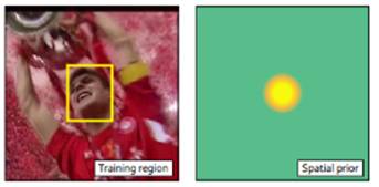
Fig. 1. Space correction
7. TRACKING ALGORITHMS
BASED ON MOSSE FILTERS
Minimum
Output Sum of Squared Error (MOSSE) uses adaptive
correlation for target tracking which produces stable correlation filters when initialised using a single frame. MOSSE
tracker is robust to variations in lighting, scale, pose, and non-rigid
deformations. It also detects occlusion based upon the peak-to-side lobe ratio,
which enables the tracker to pause and resume when the target reappears.
Starting
from a reduced set of images, we need a set of training pictures, ![]() , and their corresponding desired output
, and their corresponding desired output ![]() . In order to simplify the computations, the filters
are determined in the Fourier domain:
. In order to simplify the computations, the filters
are determined in the Fourier domain:
|
|
(18) |
In order to find the
filter that links us correctly between the desired input and output, MOSSE assumes the minimisation of
the quadratic error between the current output of the convolution between the
input and the filter and the output that is to be obtained from the
convolution.
|
|
(19) |
8. TARGET MOTION MODEL
To determine the absolute position of the
target, the position of the drone is needed and is obtained through serial
communication between the autopilot (equipped with GPS and barometer) and the
companion computer.
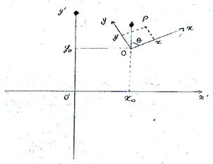
Fig. 2. Target position
from drone GPS and frame pixels
In the image above ![]() is the EARTH fixed reference, and
is the EARTH fixed reference, and ![]() is drone reference. Drone current
position in EARTH reference is
is drone reference. Drone current
position in EARTH reference is ![]() ,
, ![]() being the drone heading from the North
and
being the drone heading from the North
and ![]() target coordinates in drone reference
(Fig. 2). Then the position of the target in EARTH reference is:
target coordinates in drone reference
(Fig. 2). Then the position of the target in EARTH reference is:
|
|
(20) |
Using common mapping functions, these coordinates can be
transformed in GPS coordinates and sent to autopilot as a new waypoint. The
companion computer does this transformation and, using DRONEKIT
software (5), send the command to the drone to move.
In order to minimise the energy
consumed by the drone, the system first computes if the target movement is
likely to get the target out of the FOV (Field of
View) of the onboard camera. Only if this is true, a move command is sent to
the drone, else the drone will remain in hover, tracking the target.
Using a stabilised gimbal, the
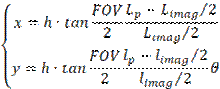
camera is always pointed downward to the EARTH. Knowing the camera resolution, ![]() focal length f and altitude of the drone
focal length f and altitude of the drone ![]() we
can compute image footprint on the ground
we
can compute image footprint on the ground ![]() , in cm/pixel.
, in cm/pixel.
From the image processing module, we get the target centre position in the frame (in pixels) ![]() . Then, the position of the target in drone
reference is given in Fig. 3:
. Then, the position of the target in drone
reference is given in Fig. 3:
|
|
(21) |
It is possible to estimate the speed of the target relative
to the drone using several such computations over short time intervals. Next,
using simple kinematics, o predicted target position can be obtained with:
|
|
(22) |
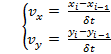
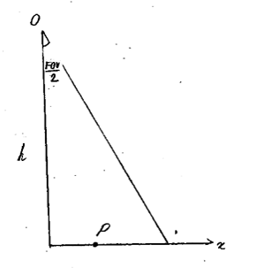
Fig. 3. Target relative position
It is possible to estimate the speed of the target relative
to the drone using several such computations over short time intervals. Next,
using simple kinematics, o predicted target position can be obtained with:
|
|
(23) |
Predicted values obtained can be sanctioned by real values
from the image tracking and prediction accuracy can be improved using an EKS (Extended Kalman Filter).
9. EXPERIMENTAL SETUP
For the experiments, video captures where registered from
the drone at various altitudes and illumination conditions, both the in urban
and rural context.
The selected UAS is a quadcopter (Fig. 4) due to its
agility in flight and mechanical simplicity, ability to keep flying over the
target in a stable manner while taking pictures. The quadcopter is made
entirely of carbon fibre, with 16 mm diameter tube
arms, spacing between motors centres being 650 mm.
The central rig is divided into three levels and houses the
whole system. At the top level, there is the image-processing unit, the NVIDIA
Jetson TX2. On the second level is the Pixhawk autopilot, GPS, magnetometer unit, Wi-Fi antennas
and radio telemetry modem. Level 3 houses the batteries. Under the bottom level
is the gimbal with the Sony QX10 camera. The gimbal stabilises the camera in roll and pitch. A stabilisation system and an inertial measuring unit (IMU) that commands two brushless motors control the gimbal.
The weight of the component parts is shown in the table below.
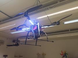
Fig. 4. Quadcopter
Tab. 1
The mass of the main components of
the experimental UAV
|
Part |
Mass [kg] |
Part |
Mass [kg] |
|
Frame |
0.61 |
Camera |
0.29 |
|
Motors |
0.39/piece |
Autopilot |
0.02 |
|
Battery |
0.80 |
Jetson TX2 |
0.10 |
|
Gimbal |
0.17 |
|
|
|
|
|
Total |
2.39 |
An 11000 mAh LiPo
(Lithium-Polymer) battery was chosen to maximise the
available electrical power while reducing weight. An electric motor 48-22-490
KV, combined with a 16x5.5 carbon fibre propeller, fulfilled the required autonomy condition.
The architecture of the electronical system is seen in Fig.
5. It consists of the Pixhawk autopilot, the
companion computer, the Jetson TX2 and the Sony QX10 camera. Pixhawk is a very
powerful autopilot, well suited for our project. It supports both human and
fully automated flight, including navigation by GPS coordinates, camera
control, takeoff and landing automatic. The video processing computer installed
on the test drone is the Jetson TX2 (6) from NVIDIA,
having the technical specifications in the table below.
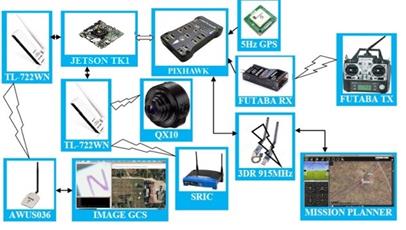
Fig. 5. System architecture
Tab. 2
Companion computer specifications
|
GPU |
NVIDIA Maxwell
™, 256 CUDA cores |
|
CPU |
Quad ARM® A57/2 MB L2 |
|
Video |
4K x 2K
30 Hz Encode (HEVC) 4K x 2K
60 Hz Decode (10-Bit Support) |
|
Memory |
4 GB 64-bit LPDDR4 25.6 GB/s |
|
Display |
2xDSI, 1xeDP1.4/DP1.2/ HDMI |
|
CSI |
up to 6 cameras (2
Lane) CSI2 D-PHY 1.1 (1.5
Gbps/Lane) |
|
PCIE |
Gen 2 | 1x4 + 1x1 |
|
Data Storage |
16 GB eMMC, SDIO, SATA |
|
Other |
UART, SPI, I2C,
I2S, GPIOs |
|
USB |
USB 3.0 + USB 2.01 |
|
Connectivity |
Gigabit Ethernet, 802.11ac WLAN, Bluetooth |
The ground control system consists of a laptop computer for
command, control and monitoring of the unmanned aircraft. Mission Planner is an
open-source ground control application for MAVlink
based autopilots and can be run on Windows, Mac OSX,
and Linux. Mission Planner allows us to set up an aeroplane,
copter or rover to use an autopilot, plan, save missions, and view live flight
information (Fig. 6).
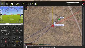
Fig. 6. Mission Planner
A second laptop computer runs the image operator console,
which monitors the tracking image processing and is used for initial choosing
of the target (Fig. 7).
10. EXPERIMENTAL RESULTS
Implementation was done in Python with the OpenCV library. Nonetheless, there are several constraints
to be considered. For example, CSRT supports an OpenCV version of more than 3.4, while the rest of the
algorithms work with OpenCV 3.2.
The table below presents a series of experimental results
obtained with the techniques presented in the previous paragraph. Experiments
were performed on the HD video stream from the SONY QX10
on the companion computer Jetson TX2.

Fig. 7. Image operator console
It was noted that the MOOSE algorithm manages to achieve
the best processing rate. However, following the experiments, it has been
demonstrated that CSRT tends to be more accurate in
terms of precision but compared to MOOSE, it is slower.
Tab. 3
Results obtained for
different algorithms
|
Method |
Video resolution |
FPS |
|
Boosting |
1280x720(HD) |
30 |
|
MIL |
1280x720(HD) |
18 |
|
KCF |
1280x720(HD) |
43 |
|
CSRT |
1280x720(HD) |
24 |
|
MOOSE |
1280x720(HD) |
72 |
Below, in Figs. 8 and 9, some snapshots were presented
during experiments on HD video. The green dial in HD images shows a successful
tracking of user-marked targets. The “Vertical”,
“Horizontal”, “Up” and “Down” labels in
blue are the directions in which the drone should move to keep the target
in FOV.
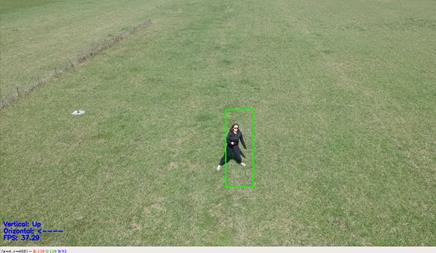
Fig. 8. Person tracking
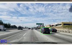
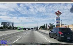
Fig. 9. Car tracking
11. CONCLUSIONS
Figure 9 shows that the
proposed method can track the target with good performance. When light changes
in Fig. 9 or occlusion occur, the accuracy rate of the proposed method is
nearly 100% if the allowable error threshold is greater than 15 pixels. When
deformation occurs, the accuracy rate of the proposed method is nearly 100% if
the allowable error threshold is greater than 5 pixels. In practical application,
the allowable error threshold of 5 pixels or 15 pixels has almost no influence
on tracking. The experiment shows that the proposed method fulfils the
requirement of tracking a moving target.
References
1.
Babenko B., M.H.
Yang, S. Belongie. 2009. Visual Tracking with
Online Multiple Instance Learning. CVPR.
2.
DRONEKIT. „Developer Tools for Drones”. Available at: https://github.com/dronekit/dronekit-python.
3.
Grabner Helmut, Grabner Michael, Bischof Horst.
2006. “Real-time tracking via
on-line boosting”. Proceedings
of the British Machine Vision Conference 1: 1-10. ISBN 1-901725-32-4. DOI:10.5244/C.20.6.
4.
Henriques J.F.,
R. Caseiro, P. Martins, J. Batista. 2015. “High-Speed Tracking with Kernelized
Correlation Filters”. IEEE
Transactions on Pattern Analysis and Machine Intelligence 37(3): 583-596.
5.
Jetson TX2. „High Performance AI at
the Edge”. Available at: https://www.nvidia.com/en-us/autonomous-machines/embedded-systems/jetson-tx2.
6.
Lukežič Alan, Tomáš Vojíř,
Luka Čehovin, Jiří
Matas, Matej Kristan. 2018. “Discriminative Correlation Filter Tracker with Channel and Spatial
Reliability”. International
Journal of Computer Vision 126(7): 671-688. DOI: 10.1007/s11263-017-1061-3.
7.
Mukesh kiran
K, Nagenra R. Velaga, RAAJ Ramasankaran. 2015. “A
two-stage extended kalman filter algorithm for
vehicle tracking from GPS enabled smart phones through crowd-sourcing”. European Transport \ Trasporti
Europei 65(8). ISSN: 1825-3997.
Received 20.09.2019; accepted in revised form 27.10.2019
![]()
Scientific
Journal of Silesian University of Technology. Series Transport is licensed
under a Creative Commons Attribution 4.0 International License