Article
citation information:
Dogan, E., Korkmaz, E., Akgungor,
A.P. Comparison
of different approaches in traffic forecasting models for the D-200 highway in
Turkey. Scientific Journal of Silesian
University of Technology. Series Transport. 2018, 99, 25-42. ISSN: 0209-3324. DOI: https://doi.org/10.20858/sjsutst.2018.99.3.
Erdem DOGAN[1],
Ersin KORKMAZ[2], Ali Payidar AKGUNGOR[3]
COMPARISON OF
DIFFERENT APPROACHES IN TRAFFIC FORECASTING MODELS FOR THE D-200 HIGHWAY IN
TURKEY
Summary. Short-term traffic estimations have a significant
influence in terms of effectively controlling vehicle traffic. In this study,
short-term traffic forecasting models have been developed based on different
approaches. Seasonal autoregressive integrated moving average (SARIMA), artificial
bee colony (ABC) and differential evolution (DE) algorithms are the techniques
used in the optimization of models, which have been developed by using
observation data for the D-200 highway in Turkey. 80% of the data were used for
training, with the remaining data used for testing. The performances of the
models were illustrated with mean absolute errors (MAEs), mean absolute
percentage errors (MAPEs), the coefficient of determination (R2) and the
root-mean-square errors (RMSEs). It is understood that all the models provided
consistent and useful results when the developed models were compared with the
statistical results. In the models created separately for two lanes, the R2
values of the models were calculated to be approximately 92% for the right
lane, which is generally used by heavy vehicles, and 88% for the left lane,
which is used by less traffic. Based on the MAE and RMSE values, the model
developed by the ABC algorithm gave the lowest error and showed more effective
performance than the other approaches. Thus, the ABC model showed that it is
appropriate for use on other highways in Turkey.
Keywords: traffic forecasting;
SARIMA; differential evolution algorithm;
artificial bee colony algorithm
1. INTRODUCTION
The increase in travel demand causes an increase in traffic density. This
situation requires traffic management to be carried out more efficiently. Thus,
people can travel more efficiently since warnings and instructions for the
drivers will be reduced as a consequence. Being aware of current and expected
traffic conditions is of critical importance in the decision-making process.
Therefore, many researchers have used different approaches to forecast
short-term traffic flow.
The Box-Jenkins technique is one of the cornerstone statistical methods,
which has been applied in short-term traffic forecasting [1]. Since its
introductions, different algorithm approaches have been used to study this
subject. For example, Chrobok et al. [2] used traffic data obtained over two
years with the help of 350 detectors in Duisburg, a city in Germany. Traffic
flow data were collected at 1-min intervals and divided into four different
groups via the developed method. As a result, they found that intuitive models
showed better results in long-term traffic forecasting, while linear models
showed better results in short-term traffic forecasting. Zhong et al. [3]
developed a time-delayed artificial neural network (ANN) and genetically
designed regression models for traffic predictions with regard to different types
of roads via data obtained from rural roads. Hourly, daily and seasonal
forecasting models have been developed for traffic data and compared using
different period data. It has been found that the weighted regression model
gives better results. Vlahogianni et al. (4) conducted a short-term traffic
forecasting study using an ANN on a road corridor where there are intersections
with traffic signals. The authors indicated that the ANN gave the best results
for predictions in light of previous studies, which preferred to optimize ANN
weights by a genetic algorithm (GA) according to different road
characteristics. Researchers have developed ANN architectures by using two
types of inputs, namely, univariate and multivariable. Ultimately, they pointed
out that the GA-optimized ANN offers potential to forecasting models. Jiang et
al. [5] tried to make traffic forecasts on a daily and hourly scale by creating
a dynamic wavelet ANN model. Researchers have indicated that this model is a
powerful approach for acquiring traffic flow; furthermore, it uses the
“Mexican hat wave” to improve the model. Lam et al. [6] estimated
the average daily traffic value with the help of two non-parametric models. The
Gaussian maximum likelihood (GML) and non-parametric regression (NPR) models
are presented with the help of information obtained from 87 counting stations.
It has been stated that the NPR model provides more accurate results than the
GML model for most stations. Another result from this study was that the NPR
model is better at adapting to sudden and unexpected traffic flow conditions.
Zhang and Ye [7] used the fuzzy logic (FL) model to estimate short-term traffic
flow. Previously used traffic flow forecasting methods are the Kalman filter
(KF), the exponential smoothing method (ESM), backpropagation neural networks
(BPNNs) and the autoregressive integrated moving average (ARIMA), which were
applied in order to generate input parameters for the FL model. When the
proposed model was compared with existing methods, using dual-loop data
collected from I-35 in San Antonio City, Texas, the fuzzy logic system was
found to make more accurate and stable predictions. Shekhar and Williams [8]
designed the SARIMA model so that it could adapt to new seasonal data. They
compared the 15-min traffic forecast values of this model and the other models
including KF, recursive least squares and least mean squares. As a result, all
models provided consistent results, while it has been proposed that the
developed SARIMA model should provide convenience to intelligent transport
system applications in the field. Castro-Neto et al. [9] developed the online
support vector machine (OL-SVM) method to estimate traffic flow in typical and
atypical traffic conditions. The accurate prediction of the models has been
assessed according to two different scenarios. In the first scenario, which is
considered as typical traffic conditions, three working days a week were
examined. On the other hand, in the second scenario, which considers atypical
traffic conditions, holidays and days when traffic accidents occurred were
examined. The proposed model has been compared to three different prediction
models: GML, Holt exponential smoothing and ANN models. It is seen that the GML
model made more effective predictions in the first scenario. It is emphasized
that the developed OL-SVM model provides more accurate results than the other
methods in the second scenario. Zargari et al. [10] performed short-term
traffic forecasting using three different computational intelligence techniques,
namely, linear genetic programming (LGP), multilayer perceptron (MLP) and FL.
All models have been developed for the traffic flow rates in the 5-min and
30-min time intervals. LGP and MLP models provide consistent results; and, in
general, these results are reported as better than FL results. Another result
is that the 30-min estimates are better than the 5-min estimates. Hong et al.
[11] attempted to estimate traffic flow by using the support vector regression
(SVR) and the ant colony optimization (ACO) methods. The results of this study
have also been compared with the predictions of the SARIMA model. Researchers
have reported that the hybrid model was not only better than the SARIMA model
but could easily be used in traffic control centres. Xia et al. [12] developed
an algorithm that identifies online traffic situations. This method, which
works with 5-min data on traffic flow, density and speed, tries to classify
next 1-min data. The developed method has been tested on two different
highways, with test results showing that the identified freeway traffic states
via the proposed procedure were reasonable and consistent. Tchrakian et al.
[13] used the spectral analysis technique to estimate the 15-min short-term
predictions for traffic with real-time updating. Therefore, they sought
predictions for within-day traffic flow using a forecasting horizon of 1 h and
15 min in 15-min steps. They indicated that the technique combines the features
of a time series-based prediction with spectral analysis, which is appropriate
for estimations in low-frequency modes. Guo et al. [14] performed data
smoothing with a single spectrum analysis method for better short-term traffic
estimation. Smoothed data have been utilized in a novel prediction method known
as the grey system model (GSM) to predict traffic flows on urban roads. The new
model has been compared to the SARIMA model in the context of corridor data
from Central London. As a result, it has been reported that better results are
obtained when smoothing is applied.
Recently, artificial intelligence methods, such as ANN, DE and ABC
algorithms, have been used in engineering and transportation problems. Even
though ABC and DE algorithms are not used in traffic estimation, they have been
applied to address many issues, such as signal optimization and delay, with
successful results obtained. The ANN method has been used in the estimation of
delay and vehicle stops at signalized intersections by Doğan et al. [15],
while Dell’Orco et al. [16,17] applied the ABC and harmony search
algorithms to traffic signal optimization. The method, based on the harmonic
search algorithm, has produced effective and simpler optimization results. In
addition, it has been shown that the ABC method improves the performance index
by 2.4- 2.7% in comparison with the GA and the hill climbing algorithm. Yunrui
et al. [18] examined the traffic signal control with the DE algorithm, stating
that it was effective in determining system parameters and the results were
good enough to reduce delay, queue length and parking ratio. Lin [19] used this
technique to resolve transport problems with fuzzy coefficients and showed that
the results were as effective as GAs in solving transportation problems.
Artificial intelligence methods are also widely used in image analysis [20-27],
which is applied in the optimization of transport processes.
In this article, models based on SARIMA, ABC and DE
algorithms will be presented, and the performance of different approaches will
be shown. The absence of traffic estimation studies, based on ABC and DE
algorithms, distinguishes this article from other studies. In the second
section of the paper, the methods to be used in developing the models will be
explained. Additionally, traffic flow data used to develop models will be
briefly explained in the same section. After testing the developed models,
which will be mentioned in the next section, the generated values will
presented in the findings section. The results and proposals for further
studies are given in the last section.
2. METHODOLOGY
2.1. Traffic flow data
The traffic count was
carried out on the D-200 highway, which is on the border of
Kırıkkale, in the Turkish interior. The city is an important point
linking 35 cities to each other. The D-200 state road, where the study was
conducted, is a two-way, two-lane highway. There were no factors (e.g.,
signalized intersections or entrance link.) that could have cut off the main
road traffic for 20 km in the forward and backward directions in the
measurement section of the D-200 highway with two platforms. For this reason,
uninterrupted flow conditions prevailed in the section where the count was
made. The counting process was carried out with NC-350 traffic counting devices
placed separately on the right and left lanes in a one-way direction. Each
count represented a 15-min period. At the end of the count, a total of 4,512
data items were collected. Since the data collection and battery capacity of
the counting devices were limited, the data collection process was completed
with three separate counting studies. Time losses due to device changes between
each counting study and other unknown reasons caused interruptions in data
collection. The missing data was completed, as shown in Fig. 1, by taking data
from the previous week for the same day and time. In this way, the incomplete
amount of data, equivalent to less than 1% of the total amount, was practically
completed.
Among the examined
dates, a daily average of 8,627 vehicles was counted for the right and left
lanes. The maximum number of vehicles was 720 vehicles/s for the right lane and
684 vehicles/h for the left lane. Approximately 27% of the vehicles using the
right lanes and 16% using the left lanes were heavy vehicles.
2.2. Seasonal
autoregressive integrated moving average
The autoregressive
integrated moving average (ARIMA) method is used in the analysis of time series
and predicting future values. The first basic characteristic of the method was
described by Peter Whittle in 1951, but was popularized in 1971 with a book
published by Box and Jenkins [28]. In the ARIMA method, values of any given
time in its series are indicated by a linear eq. consisting of values for the
previous period and errors made in estimation terms. It is accepted that the
average of the series used in the model is ‘0’ and that variance is
constant throughout the series, that is, the series is stationary. For
non-stationary series, previous values of the series can be stabilized by
taking the differences as shown in Eq. 1. This is known as a stationary
process. In Eq. 1, Δ is called the difference operator. The difference
operation is performed according to this equation, while the delay value is 1.
The difference operation for delay value 2 is given in Eq. 2.
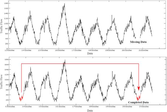
Fig.
1. Completion of missing data
![]() (1)
(1)
![]() (2)
(2)
In
the ARIMA models, the lag operator (L) is used to simplify the expression of
the stationary process as an equation. The lag operator is defined as per Eq.
3.
![]() (3)
(3)
ARIMA
(p, d, q) models consist of two main parts: autoregressive (AR) and moving
average (MA) parts. The AR part expresses the relation between the time series
and previous time values. The level of this relationship is shown as AR (p). MA
(q) represents the error terms for the prediction. ARMA (p, q) can be expressed
in terms of AR (p) and MA (q) in Eq. 4.
![]() (4)
(4)
where xt and εt are
the actual value and random error at time period t, respectively.
The
seasonal ARIMA representation is SARIMA (p, d, q) (P, D, Q)s. The general
notation with the lag operator (L) is given in Eq. 5.
![]() (5)
(5)
where:
![]() -
AR polynomial
-
AR polynomial
![]() -
seasonal AR polynomial (SAR)
-
seasonal AR polynomial (SAR)
![]() -
MA polynomial
-
MA polynomial
![]() -
seasonal MA polynomial (SMA)
-
seasonal MA polynomial (SMA)
![]() - difference and seasonal difference,
respectively
- difference and seasonal difference,
respectively
2.3. Differential
evolution algorithm
The DE algorithm, which
was introduced by Storn and Price [29], is a population-based and intuitive
approach with a working principle close to the GA. The DE algorithm, which is
basically based on the GA, has a structure consisting of four basic steps. In
other words, simple arithmetic operators in the DE algorithm are combined with
traditional operators in the GA. These basic steps are initial population,
mutation, crossover and selection. However, some existing operational
differences distinguish this algorithm from the GA. Using real-value variables
and having a different mutation process are some of the most important
differences between them. In the mutation operator of the DE algorithm,
differences between randomly selected vectors are used so that the appropriate
step size can be determined using these differences. This situation makes the
mutation operator adaptive. The algorithm’s mutation operator improves
its performance and makes it stronger. In addition, not all operators are
applied to the whole population as in the case of the GA, while these
operations are performed on randomly selected chromosomes. In brief, a
fundamental difference with the DE algorithm involves the technique of creating
the trial vector by combining the weighted difference vector with the base
vector. What should be noted here is that enough diversity should be provided
to the population to avoid early convergence. The DE algorithm can be
controlled with fewer parameters including the step size (F), the crossover
probability constant (CR) and the population size (NP).
The most important part
of any heuristic search method is to create the initial population. The best
result can be found and the convergence can be done quickly when the initial
population is correctly created. The number of input variables (D) is
determined by the size of each chromosome, while the number of chromosomes in
the population is determined by the user. The population size (NP) cannot be
less than 3 since at least three different chromosomes are needed to obtain the
difference vector and the base vector. The initial population is determined by
the upper and lower bounds of the parameters. The mathematical expression of
the initial population is given in Eq. 6.
![]() (6)
(6)
where ![]() are the upper and lower bounds of the
j-th parameter.
are the upper and lower bounds of the
j-th parameter.
Usually, one or two difference
vectors are used in the mutation operator. If one difference vector is used,
the mathematical expression is shown in Eq. 7.
![]() (7)
(7)
where ![]() is the
mutant vector,
is the
mutant vector, ![]() is the
base vector, G is generation number, F is the scaling constant,
is the
base vector, G is generation number, F is the scaling constant, ![]() and
and ![]() are
randomly selected vectors to produce the difference vector.
are
randomly selected vectors to produce the difference vector.
In the mutation
operator, DE uses many different strategies: DE/best/1/exp, DE/rand/1/exp,
DE/best/2/exp, DE/rand/2/exp, DE/best/1/bin, DE/rand/1/bin, E/best/2/bin, DE/rand/2/bin,
where rand or best refers to a base vector, 1 or 2 is the number of difference
vectors, and exp or bin is the type of crossover. In the crossover operator,
the trial vector is obtained via a combination of the mutant vector and the
target vector. One of the three different crossover methods and CR are used in
this process. These methods are binomial, exponential and arithmetic. In the
binary crossover method, the vectors forming the test vector are selected from
the mutant vector and the target vector by the crossover rate. The choice of
each vector is independent of each other. The aim is to prevent the trial
vector from being a duplication of the target vector and to force one of the
vectors forming the trial vector to come from the mutant vector. The expression
of the crossover method under these conditions is given by Eq. 8.
 (8)
(8)
where ![]() is the trial vector and
is the trial vector and ![]() varies from 0 to 1, according to the
uniform distribution, and
varies from 0 to 1, according to the
uniform distribution, and![]() ranges from 1 to D.
ranges from 1 to D.
In the
exponential method, the crossover is similar to the crossover operator at one
or two points, and it is the same as the crossover used in this genetic
algorithm. The expression for the exponential crossover method is given by Eq.
9.
 (9)
(9)
where n is the random integer between 1 and D, and (n) D is the
remainder of n/D.
The arithmetic crossover, as
expressed by Eq. 10, is the result of an arithmetic combination of the target
vector and the mutant vector.
![]() (10)
(10)
where q is the weight coefficient that regulates the equilibrium between
the mutant vector and the target vector.
The
creation of a new generation occurs in the selection operator, which is the
last operation of the DE algorithm. It creates a new generation by making the
best choice between the test vector and the target vector to minimize the
fitness function. The expression for the selection operator is given by Eq. 11.
 (11)
(11)
In their
study, Mallipeddi et al. confirmed the optimum range for the DE, NP, CR and F
parameters, stating that it should be between 4D and 10D for NP, between 0.9
and 1 for CR, and between 0.4 and 0.95 for F [30].
2.4. Artificial bee
colony algorithm
In
2005, Karaboğa [31] developed the ABC algorithm by modelling the food
search behaviour of bees. Karaboğa made some assumptions in order to make
the algorithm simpler in the development process. In his assumptions, every
source in the solution space is used by an employed bee and the number of
employed bees in the population is equal to the number of onlooker bees. Thus,
each source that refers to the solution of the problem and the amount of food
in the source also indicate the suitability of the solution. In this case, the
point that expresses the minimum or the maximum value for the problem is the
source that has the most nectar. At the beginning of the algorithm, the food
sources are searched by the scout bees, then the nectars are collected from
these sources. Therefore, the bees returning to employment, after scouting has
ended, carry the nectar to the hive and share the source information with
onlooker bees. While onlooker bees move towards rich sources, according to the
shared information, employed bees leave the depleted sources. Employed bees
returning from depleted sources are classified as scout bees given that they
investigate new sources. This situation continues over a number of cycles until
an optimum solution is found. The high performance of the algorithm is only
possible if the initial source is created correctly. In this respect, it is
essential that the sources corresponding to the solutions, including the entire
search space, are randomly determined. In this regard, the sources representing
the solution points need to be determined at random. The mathematical
expression of initial sources is given in Eq. 12.
![]() (12)
(12)
where ![]() creates a source, and
creates a source, and ![]() refer to the lower and upper limits of
each parameter.
refer to the lower and upper limits of
each parameter.
There are
searches for new sources in the neighbourhood of the initial one, which
randomly creates sources. The mathematical expression for seeking the new
sources is given in Eq. 13.
![]() (13)
(13)
where ![]() is an existing food source,
is an existing food source, ![]() represents new resources sought in the
neighbourhood of the existing resource,
represents new resources sought in the
neighbourhood of the existing resource, ![]() is a random number varying between -1 and
1, and
is a random number varying between -1 and
1, and ![]() represents a randomly selected
neighborhood solution. Decreasing the difference between
represents a randomly selected
neighborhood solution. Decreasing the difference between ![]() provides the optimum solution. There are
boundaries for
provides the optimum solution. There are
boundaries for ![]() in expressing the source of the
neighbourhood; and, if these boundaries are violated,
in expressing the source of the
neighbourhood; and, if these boundaries are violated, ![]() is again shifted between these
boundaries. These boundaries are given in Eq. 14.
is again shifted between these
boundaries. These boundaries are given in Eq. 14.
 (14)
(14)
The
calculation of the quality of new resources is carried out as a result of
finding new sources within the limit values. The mathematical expression of the
fitness function is given in Eq. 15.
![]() (15)
(15)
where the value of ![]() is the cost value of neighborhood
resource
is the cost value of neighborhood
resource ![]() .
.
The
choice between the existing source and the new source is made by performing a
greedy selection process according to the fitness values of the resources.
Since the selection process is performed according to a roulette wheel, the
sharing of each region in wheel is determined. The expression for the
probability of the selection function is given in Eq. 16.
![]() (16)
(16)
where ![]() is the fitness value of i and
is the fitness value of i and ![]() is the probability of selection.
is the probability of selection.
3. DEVELOPMENT OF THE MODELS
80% of the 4,512 traffic data items collected from
the D-200 highway were used in developing models, with the remaining data used
for testing. Different traffic flow prediction models were developed using the
SARIMA, ABC and DE methods depending on the training data. These models are discussed
in detail below.
3.1. Seasonal autoregressive
integrated moving average traffic flow forecasting model
In order to develop the SARIMA model for traffic flow data, the variance
must be constant and the average must be ‘0’. In addition, the data
set must be stationary. Autocorrelation is used to determine the stability of
the time series. The autocorrelation function (ACF) can be defined as the
correlation function between the values of a time series at different times.
The Box-Jenkins method [28] has been used to determine the model. In Fig. 2,
the ACF and the partial ACF (PACF) are shown for right and left lanes. These
functions are used for determining the AR and MA degrees.
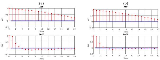
Fig.
2. Right (a), left (b) ACF and PACF values
The
slow decrease in ACF values in Fig. 2 for both lanes indicates that the series
is not stationary. For this reason, the series has been stabilized by applying
difference procedures. In Fig. 3, it is observed that the ACF and PACF values
are cut off at the first delay value for both lanes. This indicates the state
of MA (1). It is also revealed that the series has negative ACF values, which
indicates the state of SMA (672). The appropriate time series model is expected
to occur in SARIMA (0,1,1) (0,1,1)672.

Fig.
3. ACF, PACF and lags of traffic flows after stabilization
In addition to the model
indicated by the Box-Jenkins method, ARIMA and SARIMA models with different
structures have been developed for comparison purposes. The model types used for comparison and
the mean squared errors (MSEs), as shown in Eq. 17, for estimations are given
in Tab. 1.
![]() (17)
(17)
where tfobserved is actual traffic flow values and tfestimated
is the model’s traffic flow forecast value.
Tab.
1.
Mean squared errors of models for test data
|
No. |
ARIMA |
MSE right |
MSE left |
No |
SARIMA |
MSE right |
MSE left |
|
1 |
(0,1,1) |
3243.2 |
955.5 |
6 |
(0,1,1) (0,1,1)96 |
234.92 |
337.5 |
|
2 |
(0,1,2) |
3559.0 |
954.5 |
7 |
(0,1,1) (0,1,1)672 |
526.24 |
236.1 |
|
3 |
(1,1,0) |
3243.2 |
955.5 |
8 |
(0,1,1) (1,0,1)96 |
3024.5 |
983.7 |
|
4 |
(1,1,1) |
2971.5 |
918.7 |
9 |
(0,1,1) (1,0,1)672 |
233.51 |
119.7 |
|
5 |
(1,1,2) |
2959.1 |
915.8 |
10 |
(1,0,1) (0,1,1)96 |
153.41 |
138.5 |
|
|
|
|
|
11* |
(1,0,1) (0,1,1)672 |
94.38 |
64.66 |
|
|
|
|
|
12 |
(1,1,1) (1,1,1)96 |
236.78 |
314.1 |
|
|
|
|
|
13 |
(1,1,1) (1,1,1)672 |
223.55 |
170.9 |
The
lowest MSE values of 94,38 and 64,66 were observed in the SARIMA (1,0,1)
(0,1,1)672 model. The SARIMA model proposed according to the Box-Jenkins method
had a worse performance. When the ACF and PACF values of the SARIMA (1,0,1)
(0,1,1)672 model are examined, it is understood that this model should be used
because there is no correlation in the series and it has low MSE values. The
general expression of this model for the right and left lanes is given by Eqs. 18-19,
respectively.
![]() (18)
(18)
![]() (19)
(19)
3.2. Artificial bee
colony and differential evolution traffic flow forecasting models
Traffic
flow forecasting models developed using ABC and DE algorithms are presented in
three different forms, with these models optimized using the proposed
algorithms. The traffic data belonging to the previous time series are used as
model parameters. These traffic data are the number of vehicles belonging to
the times that are 1 h before the time when short-term traffic flow is
predicted. These model forms have been selected in this study as linear,
semi-quadratic and power form. The expressions of these forms are given in Eqs.
20-22.
Linear form:
![]() (20)
(20)
Semi-quadratic form:
![]() (21)
(21)
Power form:
![]() (22)
(22)
where X1
is the number of vehicles in time t-60, X2 is the number of vehicles
in time t-45, X3 is the number of vehicles in time t-30, X4
is the number of vehicles in time t-15, and Wi values are coefficient values
related to equations.
The
important point with these models is the number of independent variables used
in the form of the equations. The use of four different traffic data items
obtained 1 h before the desired time ensures that the model is more consistent.
The use of more parameters is not preferred as it will cause the models to move
away from practicality. There has been an attempt to use the most optimal
number of independent parameters since the use of fewer parameters will also
move the model away from accuracy. Coefficient values of models optimized by
the DE and ABC approaches are found according to training data. Each approach
used in the determination of coefficient values requires control parameter
values, so that the algorithm can perform the operators and reach the optimum
solution. The parameter values used in the DE algorithm are given in Tab. 2.
Tab.
2.
Control parameters of the DE algorithm
|
Population
size (Np) |
30 |
|
Crossover
state (CR) |
0.90 |
|
DE step
size (F) |
0.95 |
|
Mutation
strategy |
DE/best/1/exp |
|
Maximum
number of iterations |
1,000 |
These
values, as used in the DE algorithm, have been chosen according to the optimum
intervals determined by Mallipeddi et al. [30]. As a result of the analysis
using different parameter values, it is understood that there is no difference
between the coefficients of the model; rather, there is only a difference in
the number of iterations used to find the optimum solution. The control
parameters used in the ABC algorithm are given in Tab. 3.
Tab.
3.
Control parameters of ABC algorithm
|
Number of
bees in the colony (Np) |
50 |
|
Number of
food sources |
Np/2 |
|
Number of
sources depleted by bees |
100 |
|
Maximum
number of iterations |
1,000 |
The
coefficients of the models for the right and left lanes are given in Tabs. 4-5.
Tab.
4.
DE model coefficients
|
Right lane |
Left lane |
||||
|
Linear |
Power |
Semi-quadratic |
Linear |
Power |
Semi-quadratic |
|
w1=0.0006 |
w1=1.151 |
w1=-0.018 |
w1=-0.008 |
w1=1.043 |
w1=-0.310 |
|
w2=0.154 |
w2=0.022 |
w2=-0.145 |
w2=0.104 |
w2=0.203 |
w2=-0.059 |
|
w3=0.325 |
w3=0.178 |
w3=-0.159 |
w3=0.339 |
w3=0.232 |
w3=0.148 |
|
w4=0.490 |
w4=0.185 |
w4=-0.541 |
w4=0.525 |
w4=0.139 |
w4=0.480 |
|
w5=1.890 |
w5=0.584 |
w5=0.603 |
w5=0.878 |
w5=0.415 |
w5=0.164 |
|
|
|
w6=-1.169 |
|
|
w6=0.324 |
|
|
|
w7=1.105 |
|
|
w7=0.116 |
|
|
|
w8=0.848 |
|
|
w8=0.118 |
|
|
|
w9=-0.860 |
|
|
w9=0.041 |
|
|
|
w10=1.827 |
|
|
w10=-0.061 |
|
|
|
w11=2.330 |
|
|
w11=1.161 |
Tab.
5.
ABC model coefficients
|
Right lane |
Left lane |
||||
|
Linear |
Power |
Semi-quadratic |
Linear |
Power |
Semi-quadratic |
|
w1=0.0006 |
w1=1.187 |
w1=0.185 |
w1=-0.009 |
w1=1.167 |
w1=-0.151 |
|
w2=0.154 |
w2=-0.009 |
w2=-0.085 |
w2=0.104 |
w2=0.001 |
w2=0.008 |
|
w3=0.325 |
w3=0.142 |
w3=0.081 |
w3=0.340 |
w3=0.101 |
w3=0.115 |
|
w4=0.490 |
w4=0.335 |
w4=-0.032 |
w4=0.528 |
w4=0.331 |
w4=0.469 |
|
w5=1.890 |
w5=0.493 |
w5=-0.022 |
w5=0.878 |
w5=0.527 |
w5=-0.067 |
|
|
|
w6=-0.500 |
|
|
w6=0.237 |
|
|
|
w7=0.129 |
|
|
w7=0.128 |
|
|
|
w8=0.280 |
|
|
w8=0.233 |
|
|
|
w9=0.210 |
|
|
w9=0.010 |
|
|
|
w10=0.728 |
|
|
w10=-0.018 |
|
|
|
w11=1.650 |
|
|
w11=1.025 |
4. RESULTS AND DISCUSSION
In order to demonstrate
the accuracy of the models, the findings of the models have been compared and
performance assessments have been carried out. In this evaluation, RMSEs, MAEs,
MAPEs and the coefficient of determination R2 have been selected as
performance criteria. Mathematical expressions of performance criteria are
given in Eqs. 23-26.
![]() (23)
(23)
![]() (24)
(24)
![]() (25)
(25)
![]() (26)
(26)
The
statistical results of the developed models are given in Tabs. 6-8.
Tab.
6.
Statistics
for the SARIMA model
|
|
SARIMA |
||||
|
Test |
MAE |
MAPE |
RMSE |
R2 |
|
|
Right lane |
8.02 |
15.43 |
10.85 |
0.89 |
|
|
Left lane |
5.58 |
39.73 |
8.36 |
0.85 |
|
Tab.
7.
Training and test statistics for the DE models
|
|
Linear |
Semi-quadratic |
Power |
|||||||||
|
Test |
MAE |
MAPE |
RMSE |
R2 |
MAE |
MAPE |
RMSE |
R2 |
MAE |
MAPE |
RMSE |
R2 |
|
Right lane |
8.06 |
15.06 |
10.19 |
0.91 |
8.06 |
15.06 |
10.23 |
0.91 |
8.02 |
14.95 |
10.19 |
0.91 |
|
Left lane |
6.03 |
38.09 |
8.67 |
0.88 |
6.04 |
38.55 |
8.67 |
0.88 |
6.35 |
37.18 |
9.16 |
0.87 |
Tab.
8.
Training and test statistics for the ABC models
|
|
Linear |
Semi-quadratic |
Power |
|||||||||
|
Test |
MAE |
MAPE |
RMSE |
R2 |
MAE |
MAPE |
RMSE |
R2 |
MAE |
MAPE |
RMSE |
R2 |
|
Right lane |
8.06 |
15.06 |
10.19 |
0.91 |
8.03 |
14.87 |
10.19 |
0.91 |
8.03 |
14.89 |
10.17 |
0.91 |
|
Left lane |
6.03 |
38.08 |
8.67 |
0.88 |
6.04 |
38.12 |
8.67 |
0.88 |
6.35 |
36.93 |
8.52 |
0.87 |
When
the developed models were statistically compared, all the models showed performances
similar to each other. MAPE and R2 are scale-independent measures
and generally used to compare forecasting models [32]. The models predicted the
traffic flow with a lower error for the right lane where the traffic flow was
high, while the models for the left lane had a higher error level. The
optimized power model with the ABC algorithm especially showed the best
performance. MAPE and RMSE values of the power model were lower than those of
the SARIMA, DE and other ABC models. Therefore, the power model is the most
appropriate model for right and left lanes. The predictions of the power model,
as presented in Fig. 4, show that the power model captures the trends of
traffic flow rates throughout the day.
(a)
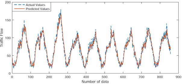
(b)
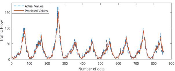
Fig.
4. The power model’s predicted and actual values: (a) right lane, (b)
left lane
6. CONCLUSION
Short-term
traffic forecasting has become an important issue, along with technologies used
in cities for traffic management, in recent years. It is now easier to estimate
future traffic with different approaches, which in turn has made managerial
decisions more efficient. Depending on the increasing number of motor vehicles
in Turkey, advanced traffic management is especially needed in major cities.
Kırıkkale, located in the Turkish interior, is an important point
linking 35 cities to each other. Thus, the data on this city, with its high
traffic intensity, were used in this study. Traffic prediction models, which
can be functionally helpful to intelligent transportation systems that likely
to be installed in these areas, were developed by using various methods. In the
development of these models, 15-min traffic flows obtained from the D-200
highway were used. Separate models for both left and right lanes were
developed, as traffic flow measurements were separately performed for both
lanes. According to the statistical results of the developed models, they all
produced consistent and useful results. However, it was observed that there
were slight differences between the models. Models showed better performance
for the right lane, which had heavier vehicles and lower speeds. Especially in
terms of MAPEs and RMSEs, the power model gave the best performance with the
lowest error rate. Therefore, the power model, when optimized with the ABC algorithm,
showed the closest results to the observation. For this reason, this model can
be used for short-term traffic forecasting in future studies. Traffic counts
could be made for two-month period to take weather changes into account [33].
It would also be useful to investigate the effect of the size of the data set
on model prediction performances after applying the counting process across the
year.
Acknowledgements
The authors would like to thank
Kırıkkale University’s Scientific Research Project Funding (KKU
BAP) for their financial support [Project No. KKUBAP2016/019].
References
1.
Ahmed M.S., A.R. Cook. 1979.
“Analysis of freeway traffic time-series data by using Box-Jenkins
techniques”. Transportation
Research Record 722: 1-9.
2.
Chrobok R., O. Kaufmann, J. Whale, M.
Schreck Enberg. 2004. “Different methods of traffic forecast based on
real data”. European Journal of Operational Research 3, 558-568.
3.
Zhong M., S. Sharma, P. Lingras. 2005.
“Short-term traffic prediction on different types of roads with
genetically designed regression and time delay neural network models”. Journal of Computing in Civil Engineering
19(1): 94-103.
4.
Vlahogianni E.I., M.G. Karlaftis, J.C.
Golias. 2005. “Optimized and meta-optimized neural networks for
short-term traffic flow prediction: a genetic approach”. Transportation
Research Part C: Emerging Technologies 13(3): 211-234.
5.
Jiang X., H. Adeli, H.M. Asce. 2005.
“Dynamic wavelet neural network model for traffic flow
forecasting”. Journal of Transportation Engineering 131(10):
771-779.
6.
Lam W.H.K., Y.F. Tang, M. Tam. 2006.
“Comparison of two non-parametric models for daily traffic forecasting in
Hong Kong”. Journal of Forecasting 192: 173-192.
7.
Zhang Y., Z. Ye. 2008. “Short-term
traffic flow forecasting using fuzzy logic system methods”. Journal of
Intelligent Transportation Systems 12(3): 102-112.
8.
Shekhar S., B.M. Williams. 2008.
“Adaptive seasonal time series models for forecasting short term traffic
flow”. Journal of the
Transportation Research Board. 2024(1): 116-125.
9.
Castro-Neto M., Y-S. Jeong, M-K. Jeong,
L.D. Han. 2009. “Online-SVR for short-term traffic flow prediction under
typical and atypical traffic conditions”. Expert Systems with
Applications 36(3): 6164-6173.
10.
Zargari S.A., S.Z. Siabil, A.H. Alavi.
2009. “A computational intelligence-based approach for short-term traffic
flow prediction”. Expert Systems 29(2): 124-142.
11.
Hong W.C., Y. Dong, F. Zheng, C.Y. Lai.
2011. “Forecasting urban traffic flow by SVR with continuous ACO”. Applied Mathematical Modelling 35(3):
1282-1291.
12.
Xia J., W. Huang, J. Guo. 2012. “A
clustering approach to online freeway traffic state identification using ITS
data”. KSCE Journal of Civil Engineering 16(3): 426-432.
13.
Tchrakian T.T., B. Basu, M.
O’Mahony. 2012. “Real-time traffic flow forecasting using spectral
analysis”. IEEE Transactions on Intelligent Transportation Systems
13(2): 519-526.
14.
Guo F., R. Krishnan, J. Polak. 2013.
“A computationally efficient two-stage method for short-term traffic
prediction on urban roads”. Transportation Planning and Technology
36(1): 62-75.
15.
Doğan E., A.P. Akgüngör, T.
Arslan. 2016. “Estimation of delay and vehicle stops at signalized
intersections using artificial neural network”. Engineering Review 36(2): 157-165.
16.
Dell’Orco M., Ö. Başkan,
M. Marinelli. 2013. “A harmony search algorithm approach for optimizing
traffic signal timings”. PROMET -
Traffic and Transportation 25(4): 349-358.
17.
Dell’Orco M., Ö. Başkan,
M. Marinelli. 2013. “Artificial bee colony-based algorithm for optimising
traffic signal timings”. Advances
in Intelligent Systems and Computing 223: 327-337.
18.
Yunrui B., D. Srinivasan, L. Xiaobo, Z.
Sun, W. Zeng. 2014. “Type-2 fuzzy multi intersection traffic signal
control with differential evolution optimization”. Expert Systems with Applications 41: 7338-7349.
19.
Lin F. 2010. “Using differential evolution for the
transportation problem with fuzzy coefficients”. In: International Conference on Technologies and Applications of Artificial
Intelligence: 299-304.
20.
Kuzhel N., A. Bieliatynskyi, O. Prentkovskis, I. Klymenko, Š.
Mikaliūnas, O. Kolganova, S. Kornienko, V. Shutko. 2013.
“Methods for numerical calculation of parameters pertaining to the
microscopic following-the-leader model of traffic flow: using the fast spline
transformation”. Transport
28(4): 413-419.
21.
Lebkowski A. 2018. “Design of an Autonomous Transport System
for Coastal Areas”. Transnav-International
Journal On Marine Navigation And Safety Of Sea Transportation 12(1):
117-124.
22.
Ogiela L., R. Tadeusiewicz, M. Ogiela. 2006. “Cognitive
analysis in diagnostic DSS-type IT systems”. In: Eighth International Conference on Artificial Intelligence and Soft
Computing (ICAISC 2006). Zakopane, Poland. Jun 25-29, 2006. Artificial Intelligence and Soft Computing -
ICAISC 2006: 962-971. Book series: Lecture
Notes in Computer Science 4029.
23.
Ogiela L., R. Tadeusiewicz, M. Ogiela. 2006. “Cognitive
computing in intelligent medical pattern recognition systems”. In: International Conference on Intelligent
Computing (ICIC). Kunming, P.R. China. 16-19 August 2006. Edited by: Huang,
D.S., Li, K., Irwin, G.W. Intelligent
Control and Automation: 851-856. Book series: Lecture Notes in Control and Information Sciences 344.
24.
Ogiela M., R. Tadeusiewicz, L. Ogiela.
2005. “Intelligent semantic information retrieval in medical pattern
cognitive analysis”. In: International
Conference on Computational Science and Its Applications (ICCSA 2005).
Singapore, Singapore. 9-12 May 2005. Edited by: Gervasi, O., Gavrilova, M.L.,
Kumar V., et al. Computational Science
and Its Applications - ICCSA 2005 Vol. 4: 852-857. Book series: Lecture Notes in Computer Science 3483.
25.
Sierpinski G., I. Celinski, M. Staniek. 2015. “The model of modal
split organisation in wide urban areas using contemporary telematic
systems”. 3rd Interntaiuonal
Conference Transportation Information Safety. Wuhan, China, Jun 25-28,
2015. P: 277-283.
26.
Smierzchalski R., A. Lebkowski. 2003. “Moving objects in the
problem of path planning by evolutionary computation”. 6th International
Conference on Neural Networks and Soft Computing. Zakopane, Poland. Jun 11-15,
2002. Neural Networks And Soft Computing.
Advances In Soft Computing: 382-387.
27.
Tadeusiewicz R., L. Ogiela, M. Ogiela. 2008. “The
automatic understanding approach to systems analysis and design”. International Journal of Information
Management 28(1): 38-48.
28.
Box G.E.P., G.M. Jenkins, G.C. Reinsel,
G.M. Ljung. 2015. Time Series Analysis:
Forecasting and Control. Hoboken, NJ: John Wiley & Sons.
29.
Storn R., K. Price. 1997. “Differential
evolution - a simple and efficient adaptive scheme for global optimization over
continuous spaces”. Journal of Global
Optimization 11(4): 341-359.
30.
Mallipeddi R., P. Suganthan, Q. Pan, M.
Tasgetiren. 2011. “Differential evolution algorithm with ensemble of
parameters and mutation strategies”. Applied
Soft Computing 11: 1679-1696.
31.
Karaboga D. 2005. “An idea based on
honey bee swarm for numerical optimization”. Technical Report - Tr06 Vol. 200. Kayseri: Computer Engineering
Department, Engineering Faculty, Erciyes University.
32.
Hyndman R.J., A.B.
Koehler. 2006. “Another look at measures of forecast
accuracy”. International Journal of Forecasting 22(4): 679-688.
33.
Calvert S.C., M. Snelder. 2016. “Influence of Weather on Traffic
Flow: an Extensive Stochastic Multi-effect Capacity and Demand Analysis”.
Transport\Transporti Europei 60(3):
1-24.
Received 07.03.2018; accepted in
revised form 29.05.2018
![]()
Scientific
Journal of Silesian University of Technology. Series Transport is licensed
under a Creative Commons Attribution 4.0 International License