Article citation information:
Šarkan, B., Skrúcaný, T., Semanová, Š., Madleňák, R., Kuranc, A., Sejkorová, M., Caban, J. Vehicle coast-down method as a tool for calculating total resistance for the purposes of type-approval fuel consumption. Scientific Journal of Silesian University of Technology. Series Transport. 2018, 98, 161-172. ISSN: 0209-3324. DOI: https://doi.org/10.20858/sjsutst.2018.98.15.
Branislav Šarkan[1],
Tomáš Skrúcaný[2],
Štefánia Semanová[3],
Radovan MADLEŇÁK[4],
Andrzej KURANC[5],
Marie SEJKOROVÁ[6],
Jacek CABAN[7]
VEHICLE
COAST-DOWN METHOD AS A TOOL FOR CALCULATING TOTAL RESISTANCE FOR THE PURPOSES
OF TYPE-APPROVAL FUEL CONSUMPTION
Summary. A coast-down test is carried out in cases when there is a need for the exact expression of the forces acting on a road vehicle during its coast-down. These forces act mainly against the vehicle’s movement due to air and tyre rolling resistance. Knowledge of the course of these forces throughout the vehicle’s movement range is also a requirement when measuring fuel consumption with a roller performance dynamometer. The reason is that this device has to load the rollers by force or performance corresponding to the given vehicle, while testing it during various driving cycles. For approval purposes, the requirements for this type of test are described in the applicable regulations, i.e., UNECE Regulations No. 83 and No. 101, or the newly developed Worldwide Harmonized Light Vehicles Test Procedure (WLTP). Slovak Technical Standard STN 30 0556 also contains detailed procedures for carrying out the test. The authors of this paper have taken into account both types of technical regulations in order to conduct coast-down tests on chosen vehicles. The results are usable in terms of measuring fuel consumption on a roller dynamometer. Furthermore, the vehicle’s economic performance in normal operation mode can be also assumed with these results.
Keywords: coast-down method, vehicle resistance, aerodynamic drag, tyre rolling resistance, fuel consumption
1. INTRODUCTION
A
coast-down test is applied to determine resistance under real conditions. This
is the test in which a vehicle running by its inertia is slowed down due to
driving resistances from the moment of shifting the neutral position of the
transmission until reaching zero speed. The test is carried out on a test
track. The driving resistances represent forces that act in opposition to the
movement of the vehicle running on a horizontal track. These include air
resistance and mechanical resistance. Air resistance is caused by the effect of
air flow as the vehicle passes through the air. Mechanical resistance
represents tyre rolling resistance and resistances in bearings and parts of the
transmission device [5 10,11,15,20].
2. measurement
methodology
The vehicle is driven on a straight
test track at constant speed under windless conditions; and, after shifting
into neutral, it moves further forward by inertia. The vehicle is thus
gradually slowed down due to rolling resistance, aerodynamic drag and friction
resistance in the transmission device until it completely stops. Changes in the
vehicle speed are continuously recorded. The vehicle movement is straight and
unevenly slowed during the coast-down. Driving resistances are calculated based
on the ascertained course of vehicle deceleration during the coast-down, as
well as geometric parameters of the test track and the known vehicle’s inertia
parameters. The coast-down characteristic of the vehicle is ascertained by
coast-down tests. Based on this characteristic, it is possible to assess the
mechanical condition of the vehicle, the chassis settings, the influence of
used tyres and the aerodynamic properties of the vehicle body [14,19].
Several requirements relating to a
vehicle, test track, test speed, atmospheric conditions and measuring equipment
must be met when carrying out coast-down tests. These requirements differ
depending on the type of regulation used. The requirements of the individual
regulations regarding a vehicle, test track, atmospheric conditions and accuracy
of the used measuring and recording equipment are listed in Table 1. The most
detailed description of such requirements is provided in the WLTP. The results
obtained in accordance with the WLTP are used for transferring the load of a
road vehicle in normal operation mode onto the rollers of a roller performance
dynamometer in order to determine the type-approval fuel consumption [25,30].
The methodology recommended by the
WLTP involves performing each coast-down measurement without interruption. However,
the division of the section is permitted if the data cannot be collected in a
continuous manner across the full speed range. When dividing the measurement
process, it is necessary to ensure that vehicle conditions remain as stable as
possible at each point of division [29].
Tab. 1
Different requirements for
carrying out the coast-down test [23,27,28,29]
|
Measurement requirements |
Available methodologies for the
coast-down |
||||
|
UNECE No. 101 |
UNECE No. 83 |
WLTP |
STN 30 0556 |
||
|
Test track parameters |
Longitudinal
slope |
±2% |
±1.5% |
±1% |
±1% |
|
Local
inclination |
±0.5% |
- |
±0.5% |
- |
|
|
Cross-sectional
slope |
Max. 1.5% |
- |
Max. 1.5% |
Max. 1.5% |
|
|
Atmospheric conditions |
Wind
speed (average) |
Max. 3 m·s-1 |
Max. 3 m·s-1 |
Max.
7 m·s-1 |
Max. 1.5 m·s-1 |
|
Wind
speed (gusts) |
Max. 5 m·s-1 |
Max. 5 m·s-1 |
Max. 10 m·s-1 |
- |
|
|
Wind
cross vector component |
Max. 2 m·s-1 |
Max. 2 m·s-1 |
Max.
4 m·s-1 |
- |
|
|
Area
of measurement above the surface |
0.7 m |
0.7 m |
- |
- |
|
|
Air
temperature |
5- 35°C |
- |
5-40°C |
5-25°C |
|
|
Air
pressure |
91-104 kPa |
- |
- |
97.33-101.25 kPa |
|
|
Relative
humidity |
Max. 95% |
- |
- |
- |
|
|
Vehicle |
Vehicle
run-in |
Min. 300 km |
Min. 3,000 km |
Min. 3,000 km |
- |
|
Tyre
run-in |
Min. 300 km |
- |
Min. 200 km |
Min. 1,000 km |
|
|
Tread
depth |
50-90% |
50-90% |
80-100% |
67% |
|
|
Time
recording (frequency) |
- |
- |
5 Hz |
- |
|
|
Measuring equipment |
Time
recording (accuracy) |
±0.1 s |
±0.1 s |
±0.01 s |
- |
|
Speed
record (accuracy) |
±0.5 km·h-1 |
±2% |
±0.5 km·h-1 |
- |
|
|
Wind
speed |
- |
- |
±0.3 m·s-1 |
- |
|
|
Wind
direction |
- |
- |
±3° |
- |
|
|
Air
temperature |
- |
- |
±1 K |
- |
|
|
Air
pressure |
- |
- |
±0.3 kPa |
- |
|
|
Vehicle
mass |
- |
- |
±10 kg |
- |
|
|
Tyre
pressure |
- |
- |
±5 kPa |
- |
|
The measurements of coast-down are
carried out in both directions repeatedly until at least three consecutive
measurement pairs meet the requirements for statistical accuracy p in percentage terms as shown below
(1).
![]() (1)
(1)
where ![]() represents the coefficient, which is
determined by the WLTP depending on the number of performed pairs of coast-down
measurements. For example, the coefficient 2.48 is used for n=3 and the
coefficient 1.6 is applied for n=4. The standard deviation expressed in seconds
is denoted as σ, while Δtj is the average time
of the coast-down at the reference speed in seconds.
represents the coefficient, which is
determined by the WLTP depending on the number of performed pairs of coast-down
measurements. For example, the coefficient 2.48 is used for n=3 and the
coefficient 1.6 is applied for n=4. The standard deviation expressed in seconds
is denoted as σ, while Δtj is the average time
of the coast-down at the reference speed in seconds.
The standard deviation is calculated according
to the following formula:
 (2)
(2)
where Δtji
represents the harmonized average time of the coast-down of the i-th pair of measurements and is
calculated according to the following formula:
 (3)
(3)
where Δtjai
and Δtjbi represent
the time of the coast-down for the i-th
measurement in each direction, respectively.
The calculated statistical accuracy of at least
three consecutive coast-down tests in each direction (three pairs of
measurements) should not exceed 3%, according to the WLTP [29].
After meeting the accuracy of the
performed coast-down tests, coast-down curves are created based on the recorded
data (Figure 1), while vehicle resistances are determined in newtons for the
whole range of examined speed. To calculate these resistances, it is necessary
to divide the coast-down curve into individual vehicle speed intervals. The
WLTP recommends an interval width of 20 km·hod-1 for the coast-down
from the speed higher, rather than 60 km·hod-1. The durations are
assigned to the respective intervals of speed decreases, and thus the vehicle
resistances are determined or the dependence of vehicle resistance on speed is
ascertained.
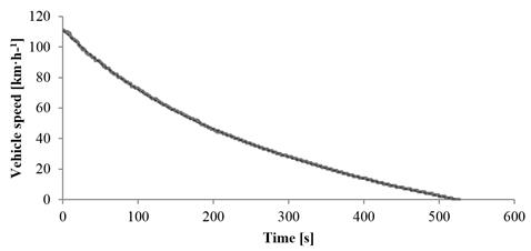
Fig. 1. Coast-down curve
The resistance force for individual
speed intervals is calculated according to the formula shown below (4). In this
formula, mav represents
the vehicle mass while tested. This is the average vehicle mass before and
after carrying out the coast-down, while considering the consumed fuel.
Further, mr is the
equivalent effective mass of all the wheels and vehicle components rotating
with the wheels during the coast-down on the road. It should be measured or calculated
by an appropriate technique. Alternatively, mr
may be estimated to be equal to 3% of the unladen vehicle mass when increased
by 25 kg.
![]() (4)
(4)
If necessary, it is also possible to
determine resistance forces for individual directions of the vehicle
coast-down. This requires calculating the average times of the intervals for
the relevant direction; however, the formula is the same as the previous one.
![]() (5)
(5)
3. Measurement results
Three
vehicles were used for practical tests on the coast-down (Figure 2). The first
tested vehicle was that used in the laboratory of the Department of Road and
Urban Transport, namely, a Kia Ceed 1.6 CVVT, which is a vehicle with a
spark-ignition engine. The vehicle kerb weight is 1,163 kg, the air resistance
coefficient is 0.33 and the vehicle frontal area is 2.25 m2. The
second tested vehicle was a Ford Galaxy 2.0 Ghia, which has a diesel engine.
The vehicle kerb weight is 1,799 kg, the air resistance coefficient is 0.314
and the vehicle frontal area is 2.78 m2. The third tested vehicle
was a Hyundai i30 Wagon with a 1.6 CRDi diesel engine. The vehicle kerb weight
is 1,413 kg, the air resistance coefficient is 0.3 and the vehicle frontal area
is 2.136 m2. Before carrying out the coast-down tests, the vehicles
were subjected to tyre pressure control and the tyres were inflated as required
by the WLTP.
|
|
|
|

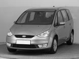

Fig. 2. Tested vehicles (Kia Ceed, Ford Galaxy,
Hyundai i30)
The
coast-down tests were carried out on the road connecting Water Dam Žilina with
the village of Mojš. The test track was 1.25 km long. The rest of the road
section was used for vehicle acceleration and turning the vehicle in opposite
direction. The road had an asphalted surface of sufficient quality. At the
beginning of the section, it was necessary to achieve the required vehicle
speed. The initial vehicle speed was 115 km·h-1 and the
coast-down was recorded from the speed of 110 km·h-1. As the test
track was not sufficiently long enough to carry out the whole coast-down, the
test was divided into two measurement parts (from 110 km·h-1 to 60
km·h-1, and from 65 km·h-1 to 0 km·h-1). The
test track is graphically illustrated in Figure 3.
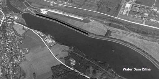
Fig. 3. Test track [Google Maps]
During the
coast-down measurements, atmospheric conditions were controlled and recorded by
using a weather station with a thermometer, a moisture meter and an anemometer.
All atmospheric conditions complied with the required level for the
measurements. The wind speed was at the average level of 1.1 m·s-1
and air temperature was 14°C.
The
universal OBD2 diagnostics device, which was compatible with the diagnostic
interface equipped with the ELM327 chip and TouchScan software, was used to
record vehicle speed over time. This device allows for recording data at a
frequency of approximately 3 Hz. Before using the diagnostics device, it is
advisable to calibrate a speed indicator, e.g., by using a roller performance
dynamometer, which is also among the equipment available from the laboratory of
Department of Road and Urban Transport [3,9,17,19]. The record of vehicle speed
over time is saved in .txt format, meaning that it is possible to work with it
in Microsoft Excel.
After
processing the results of the coast-down for tested vehicles, the calculation
of accuracy was made according to the formulas mentioned previously in the
paper (see Chapter 2). In total, three coast-down tests in each direction of
the measuring section for each tested vehicle were carried out. Each measured
coast-down was divided into two measurement parts (from 110 km·h-1
to 60 km·h-1, and from 65 km·h-1 to 0 km·h-1)
due to the insufficient length of the test track. Based on Table 2 and Figure
4, it can be concluded that the duration of the coast-down in Direction 1 was
significantly shorter than the coast-down in Direction 2. This is caused by the
longitudinal slope of the measuring section. The value of this slope was 1.1%,
which slightly exceeds the required value according to the WLTP. Therefore, the
harmonized average time
of the coast-downs was applied to the calculations. In the case of first two
vehicles, the required statistical accuracy of not exceeding 3% was met.
However, the Ford Galaxy slightly exceeded this requirement. In the case of
using this information for determining the type-approval fuel consumption or
the official measurement of fuel consumption, it would have been necessary to
repeat the measurements with this vehicle until the statistical accuracy was
achieved at the required level.
Tab. 2
Calculation of statistical
accuracy of the coast-down for the tested vehicles
|
Vehicle |
Coast-down Direction 1 [s] |
Coast-down Direction 2 [s] |
Coast-down Direction 1 [s] |
Coast-down Direction 2 [s] |
Coast-down Direction 1 [s] |
Coast-down Direction 2 [s] |
Harmonized
average time Δtji [s] |
Average time of
the coast-down Δtj [s] |
STD |
Statistical
accuracy [%] |
||
|
Kia Ceed |
145.80 |
186.28 |
145.85 |
196.02 |
145.00 |
190.30 |
163.57 |
167.25 |
164.59 |
165.14 |
1.90 |
2.85 |
|
Hyundai i30 |
143.94 |
191.25 |
149.69 |
184.75 |
147.74 |
184.36 |
164.26 |
165.38 |
164.03 |
164.56 |
0.72 |
1.09 |
|
Ford Galaxy |
149.90 |
205.77 |
150.80 |
209.70 |
153.33 |
213.89 |
173.45 |
175.44 |
178.62 |
175.83 |
2.61 |
3.68 |
It is
possible to express the resistance force of the vehicle for each direction
separately. Mainly in the case of roads with a longitudinal slope near to the
tolerance limit, or in the case of wind direction in the longitudinal direction
of the measuring section, differences may occur in the values for individual
directions. For this
reason, the harmonized average time (∆tj)
of the alternating measurements of the coast-down must also be determined, so
that the average total vehicle resistance (Fj)
can be calculated. The processed results of the coast-down test for the Hyundai
i30 are presented in detail in Table 3.
The outcome
of this type of test is the determination of the total driving resistance of
the vehicle while driving at constant speed on a horizontal road. If necessary,
it is also possible to calculate the required performance (power) to overcome
this resistance. The resultant resistance force expressed in newtons is
multiplied by the actual vehicle speed in m·s-1, such that the calculated performance required to
overcome the resistance is expressed in watts. Using these types of
calculation, it is also possible to determine the performance needed to
overcome any speed or the maximum speed of the vehicle [7,8,10,11,14,32].
Fig. 4. Average times of the coast-down in the
“there” and “back” directions for
the Hyundai i30
Tab. 3
Processed results of the
coast-down for the Hyundai i30
|
Vehicle speed and
speed intervals [km·h-1] |
Time of the
coast-down for respective intervals for Direction 1 [s] |
∆tja |
Time of the
coast-down for respective intervals for Direction 2 [s] |
∆tjb |
Fja |
Fjb |
∆tj |
Fj |
|||||
|
105 |
<110;100) |
6.17 |
6.50 |
6.14 |
6.27 |
6.69 |
7.78 |
7.24 |
7.24 |
758.52 |
657.20 |
6.72 |
707.86 |
|
95 |
<100;90) |
6.62 |
7.99 |
7.79 |
7.47 |
9.01 |
8.77 |
8.31 |
8.70 |
636.96 |
546.87 |
8.03 |
591.91 |
|
85 |
<90;80) |
8.24 |
7.87 |
8.58 |
8.23 |
9.40 |
10.10 |
10.12 |
9.87 |
577.88 |
481.70 |
8.98 |
529.79 |
|
75 |
<80;70) |
8.50 |
9.84 |
9.95 |
9.43 |
11.31 |
11.92 |
11.79 |
11.67 |
504.34 |
407.42 |
10.43 |
455.88 |
|
65 |
<70;60) |
10.80 |
11.11 |
9.96 |
10.62 |
12.94 |
12.92 |
12.82 |
12.89 |
447.69 |
368.87 |
11.65 |
408.28 |
|
55 |
<60;50) |
12.45 |
13.54 |
13.20 |
13.06 |
16.14 |
16.18 |
16.33 |
16.22 |
364.07 |
293.28 |
14.47 |
328.67 |
|
45 |
<50;40) |
13.46 |
14.50 |
14.66 |
14.21 |
18.60 |
18.14 |
18.29 |
18.34 |
334.77 |
259.27 |
16.01 |
297.02 |
|
35 |
<40;30) |
15.00 |
16.10 |
15.81 |
15.64 |
19.47 |
19.85 |
19.65 |
19.66 |
304.15 |
241.95 |
17.42 |
273.05 |
|
25 |
<30;20) |
17.45 |
17.35 |
18.02 |
17.61 |
25.76 |
25.76 |
25.76 |
25.76 |
270.12 |
184.63 |
20.92 |
227.37 |
|
15 |
<20;10) |
20.03 |
19.59 |
20.39 |
20.00 |
29.18 |
22.72 |
23.96 |
25.29 |
237.76 |
188.08 |
22.34 |
212.92 |
|
5 |
<10;0> |
25.22 |
25.30 |
23.24 |
24.59 |
32.75 |
30.61 |
30.09 |
31.15 |
193.44 |
152.68 |
27.48 |
173.06 |
|
∑ |
143.94 |
149.69 |
147.74 |
147.12 |
191.25 |
184.75 |
184.36 |
186.79 |
- |
- |
- |
- |
|
For
type-approval fuel consumption purposes, the final result of this kind of test
is the function of driving resistance curves. These curves are expressed as a
quadratic function of velocity. Individual parameters then become the basis for
transferring the load
of a particular vehicle to the rollers of a roller performance dynamometer.
Subsequently, this device is able to simulate respective driving resistances in
relation to the actual speed of a vehicle moving on the rollers.
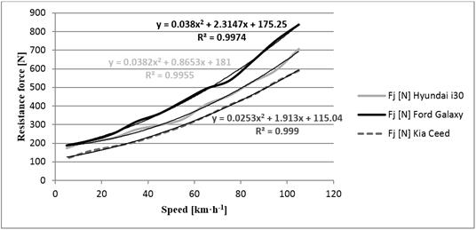
Fig. 5. Comparison of the average driving
resistance of the tested vehicles
3. Conclusion
The issue of measuring vehicle
resistance is addressed by several methodologies. For the type-approval fuel
consumption purposes in 2018, it will be necessary to follow the methodology
presented in the WLTP [20,29], which insists on significant requirements to be
met relating not only to measuring equipment but also to the test track,
atmospheric conditions and the vehicle itself. This paper has analysed the
existing regulations for carrying out the coast-down test, as well as addressed
the difficulty in quantifying driving resistances by using practical
measurement examples involving three vehicles. The difficulty of the test lies
primarily in processing the results with statistical tools in such a way that
the resultant vehicle resistance corresponds to normal operation mode as
realistically as possible.
References
1.
Barta D. 2012. Kolesové vozidlá – autobusy. Žilina: Žilinská
univerzita. ISBN 978-80-554-0644-2 [In Slovak: Wheeled Vehicles – Buses. Žilina: University of Žilina.]
2.
Barta D., M.
Mruzek, M. Kendra, P. Kordos, L. Krzywonos. 2016. “Using of non-conventional
fuels in hybrid vehicle drives”. Advances
in Science and Technology Research Journal 10(32): 240-247. ISSN 2299-8624.
DOI: 10.12913/22998624/65108.
3.
Czaban J., D.
Szpica. 2013. “Drive test system to be used on roller dynamometer”. Mechanika 19(5): 600-605. DOI:
10.5755/j01.mech.19.5.5542.
4.
Czech P. 2013.
“Intelligent approach to valve clearance diagnostic in cars”. Activities of Transport Telematics. TST
2013. Communications in Computer and Information Science 395: 384-391. DOI:
https://doi.org/10.1007/978-3-642-41647-7_47.
5.
Czech P. 2017.
“Physically disabled pedestrians – road users in terms of road accidents”. Contemporary Challenges of Transport Systems
and Traffic Engineering. Lecture Note in Networks and Systems 2: 157-165.
DOI: https://doi.org/10.1007/978-3-319-43985-3_14.
6.
Czech P. 2017.
“Underage pedestrian road users in terms of road accidents”. Intelligent Transport Systems and Travel
Behaviour. Advances in Intelligent Systems and Computing 505: 33-44. DOI:
https://doi.org/10.1007/978-3-319-43991-4_4.
7.
Drozdziel P., H.
Komsta, L. Krzywonos. 2013. “Repair costs and the intensity of vehicle use”. Transport Problems 8(3): 131-138. ISSN
1896-0596.
8.
Drozdziel P., L.
Krzywonos. 2009. “The estimation of the reliability of the first daily diesel
engine start-up during its operation in the vehicle”. Eksploatacja i Niezawodnosc - Maintenance and Reliability 41(1):
4-10. ISSN 1507-2711.
9.
Fernandez-Yaneza
P., O. Armasa, S. Martinez-Martinez. 2016. “Impact of relative position
vehicle-wind blower in a roller test bench under climatic chamber”. Applied Thermal Engineering 106: 266.
DOI: 10.1016/j.applthermaleng.2016.06.021.
10.
Figlus T., M.
Stańczyk. 2016. “A method for detecting damage to rolling bearings in toothed
gears of processing lines”. Metalurgija
55(1): 75-78. ISSN 0543-5846.
11.
Figlus T., M.
Stańczyk. 2014. “Diagnosis of the wear of gears in the gearbox using the
wavelet packet transform”. Metalurgija
53(4): 673-676. ISSN: 0543-5846.
12.
Gnap J., A.
Kalašová, M. Gogola, J. Ondruš. 2010. “The Centre of Excellence for transport
service and control”. Communications
12(3): 116-120. ISSN 1335-4205.
13.
Hockicko P., B.
Trpišová, J. Ondruš. 2014. “Correcting students’ misconceptions about
automobile braking distances and video analysis using interactive program
tracker”. Journal of science education
and technology 23(6):763-776. ISSN 1059-0145.
14.
James, D.J.G.,
K.J. Burnham, M.J. Richardson, R.A. Williams. 1999. “Improving vehicle
performance using adaptive control techniques”. Artificial Life and Robotics 3(4): 236-241. DOI:
10.1007/BF02481187.
15.
Kalašová A., Ľ.
Černický, M. Hamar. 2012. “A new approach to road safety in Slovakia”. In Transport Systems Telematics: 12th
International Conference on Transport Systems Telematics: 388-395. 10-13
October 2012, Katowice-Ustroń, Poland. ISBN 978-3-642-34049-9. Available at:
http://link.springer.com/content/pdf/10.1007%2F978-3-642-34050-5_44.pdf.
16.
Knez M., B. Jereb,
M. Obrecht. 2014. “Factors influencing the purchasing decisions of low emission
cars: a study of Slovenia”. Transportation
Research Part D: Transport and Environment 30: 53-61. ISSN 1361-9309. DOI:
10.1016/j.trd.2014.05.007.
17.
Kubíková S., A.
Kalašová, Ľ. Černický. 2014. “Microscopic simulation of optimal use of
communication network”. In Telematics –
Support for Transport. TST 2014. Communications in Computer and Information
Science: 414-423. 22-25 October 2014, Katowice- Ustroń, Poland. ISBN
978-3-662-45316-2. DOI: https://doi.org/10.1007/978-3-662-45317-9_44.
18.
Kuranc A. 2015.
“Exhaust emission test performance with the use of the signal from air flow
meter”. Eksploatacja i Niezawodnosc –
Maintenance and Reliability 17(1): 69-74.
19.
Labuda R., A.
Kovalcik, J. Repka, V. Hlavna. 2012. “Simulation of a wheeled vehicle dynamic
regimes in laboratory conditions”. Communications
14(3): 5-9. ISSN 1335-4205.
20.
Moravčík Ľ., Š.
Liščák. 2012. “Zlepšovanie legislatívy pre schvaľovanie vozidiel”. [In Slovak:
“Improvement of legislation on vehicle approval”.] In CMDTUR: Sixth International Scientific Conference: 228-243. 19-20
April 2012, University of Žilina, Žilina, Slovak Republic. ISBN
978-80-554-0512-4.
21.
Nadolski R., K.
Ludwinek, J. Staszak, M. Jaśkiewicz. 2012. “Utilization of BLDC motor in
electrical vehicles”. Przegląd
Elektrotechniczny (Electrical Review) 2012 (4a). ISSN 0033-2097.
22.
Rievaj V, P.
Faith, A. Dávid. 2006. “Measurement by a cylinder test stand and tyre rolling
resistance”. Transport 21(1): 25-28.
ISSN 1648-4142. DOI: http://dx.doi.org/10.1080/16484142.2006.9638036.
23.
STN 30 0556. Cestné vozidlá. Rýchlostné vlastnosti.
Metódy skúšok. Bratislava: Úrad pre normalizáciu, metrológiu a skúšobníctvo
SR. [In Slovak: Road Vehicles. Speed
Characteristics. Test Methods. Bratislava: Slovak Office of Standards,
Metrology and Testing.]
24.
Šipuš D., B.
Abramović. 2017. “The possibility of using public transport in rural area”. In TRANSCOM 2017: International Scientific
Conference on Sustainable, Modern and Safe Transport. Book Series: Procedia Engineering 192: 788-793. DOI: 10.1016/j.proeng.2017.06.136.
25.
TNO Innovation for
Life. Road Load Determination of
Passenger Cars. Accessed: 2 November 2017. Available at: https://www.tno.nl/media/1971/road_load_determination_passenger_cars_tno_r10237.pdf.
26.
Tomasikova M., M.
Lukac, J. Caban, F. Brumercik. 2016. “Controllability and stability of a
vehicle”. LOGI – Scientific Journal on
Transport and Logistics 7(1): 136-142. ISSN 1804-3216.
27.
UNECE. Regulation
No. 101. Uniform Provisions Concerning the Approval of Passenger Cars Powered
by an Internal Combustion Engine Only, or Powered by a Hybrid Electric Power
Train with Regard to the Measurement of the Emission of Carbon Dioxide and Fuel
Consumption and/or the Measurement of Electric Energy Consumption and Electric
Range, and of Categories M1 and N1 Vehicles Powered by an Electric Power Train
Only with Regard to the Measurement of Electric Energy Consumption and Electric
Range. Accessed: 9 November 2017. Available at:
http://www.unece.org/fileadmin/DAM/trans/main/wp29/wp29regs/2015/R101r3e.pdf.
28.
UNECE. Regulation
No. 83. Uniform Provisions Concerning the Approval of Vehicles with Regard to
the Emission of Pollutants According to Engine Fuel Requirements. Accessed: 9
November 2017. Available at:
https://www.unece.org/fileadmin/DAM/trans/main/wp29/wp29regs/r083r4e.pdf.
29.
UNECE. Global
Technical Regulation No. 15. World Harmonized Light Vehicles Test Procedure.
Accessed: 9 November 2017. Available at:
https://www.unece.org/fileadmin/DAM/trans/main/wp29/wp29r-1998agr-rules/ECE-TRANS-180a15e.pdf.
30.
UNECE. World Forum
for the Harmonization of Vehicle Regulation (WP.29).. Available at:
https://www.unece.org/trans/main/welcwp29.html.
31.
Yanowitz J., M.S.
Graboski, L.B.A. Ryan, T.L. Alleman, R.L. McCormick. 1999. “Dynamometer study
of emissions from 21 in-use heavy-duty diesel vehicles”. Environmental Science Technology 33(2): 209-216. DOI:
10.1021/es980458p.
32.
Zbigniew M., M.
Jaśkiewicz, K. Ludwinek, Z. Gawęcki. 2015. “Special characteristics of
reliability for serial mechatronic systems”. In Selected Problems of Electrical Engineering and Electronics (WZEE).
The Kielce University of Technology and The Polish Society of Theoretical and
Applied Electrotechnics – Kielce Branch. 17-19 September 2015, Kielce, Poland.
ISBN 978-1-4673-9452-9.
Received 05.11.2017; accepted in revised form 12.02.2018
![]()
Scientific Journal of
Silesian University of Technology. Series Transport is licensed under
a Creative Commons Attribution 4.0 International License