Article citation information:
Tomko, T., Puskar, M., Fabian, M., Boslai R. Procedure for the
evaluation of measured data in terms of vibration diagnostics by application of
a multidimensional statistical model. Scientific Journal of Silesian University of
Technology. Series Transport. 2016, 91,
125-131. ISSN: 0209-3324. DOI:
10.20858/sjsutst.2016.91.13.
Tomas TOMKO[1], Michal
PUSKAR [2], Michal
FABIAN[3],
Robert BOSLAI4
PROCEDURE FOR THE EVALUATION OF MEASURED DATA IN TERMS
OF VIBRATION DIAGNOSTICS BY APPLICATION OF A MULTIDIMENSIONAL STATISTICAL MODEL
Summary. The
evaluation process of measured data in terms of vibration diagnosis is
problematic for timeline constructors. The complexity of such an evaluation is
compounded by the fact that it is a process involving a large amount of
disparate measurement data. One of the most effective analytical approaches
when dealing with large amounts of data is to engage in a process using multidimensional
statistical methods, which can provide a picture of the current status of the
flexibility of the machinery. The more methods that are used, the more precise the
statistical analysis of measurement data, making it possible to obtain a better
picture of the current condition of the machinery.
Keywords: vibration diagnostics, statistical
methods
1. INTRODUCTION
From the perspective of
understanding the context of the statistical evaluation of measured data regarding
the amplitude and frequency of its engine, the Honda GX25 may experience
irregularities during the application of the statistical model. This
raises a number of important questions. Is the liner regression model suitable?
What percentage of the measured data for the statistical model can be explained
by this model? What percentage of the model is strong? Are the measured data
affected by the multicollinearity, autocorrelation or heteroscedasticity? How
much of this is determined by the normality of residues? What are the
possible errors of the model and how can they be identified? These questions are
very resolutely answered by the methodology described in this work. In the
process, these questions will also evaluate the effectiveness of the correct
application of the linear regression model with two variables using RStudio
software.
2. CALCULATION OF THE
REGRESSION COEFFICIENTS Β
The first step in
the progressive realization of the linear regression model with two variables
is to calculate the regression coefficients as follows:
![]() (1)
(1)
In view of Equation (1), it is clear that the RStudio software must
calculate an inverse matrix by multiplying the transposed matrix of matrix X by XT,
then multiplying it by the transposed matrix XT and matrix y. The
problem with Equation (1) is easy to define in the program environment of RStudio
when using the following command:
![]() (2)
(2)
This operation assures linear model parameter
estimation, which will take the shape of a vector. The output from RStudio is a
vector of estimation parameters in the following form:
3. RANDOM DISTURBANCES AND THEIR
DISPERSION IN THE FORM OF A VARIANCE–COVARIANACE MATRIX
The next step is to
define the problems of random disturbances in the environment program of
RStudio. The difficulty of this step is the fact that the variance must be
expressed in the variance-covariance matrix. From this point of view, it
is necessary to define the problem expressed by Equations (3) and (4):
![]() (3)
(3)
![]() (4)
(4)
In order for Equation
(3) to be expressed by the RStudio software, it is necessary to calculate the variance
of random values according to Equation (4). This equation refers to the proportion
by which the numerator is the product of the transposed matrix of the vector of
residual components of the ordinary matrix vector eT of residuals e. In the
denominator, the number of explanatory variables needs to increase by one. Then
the coefficient is subtracted from the number of
observations n. This problem can be defined in the
RStudio software in the following form:
![]() (5)
(5)
In this case, I used the generic
function resid (), which comes with a
standard offer RStudio program environment. This feature was chosen because of
the purpose in calculating the residual component of the regression model
itself. In addition to the generic function resid
(), I used another generic function, i.e., dim (), in this step [1]. This function determines the number of
rows of a matrix with dimension n,
while the number of columns is provided by using the dimension in relation
to k+1. The outcome of the RStudio
program is based on the defined command to estate the variance of random
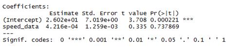
failures, as presented in (5). In this case, its value equates to 7.019. After
successfully estimating the variance of random failures, I then defined the
problem of S2 (3) using the RStudio environment program. Since this software
understands the calculated variance matrix, a scalar variable is not so
necessary in this step in order to express this matrix in scalar form. This
transformation takes place within the defined RStudio program, using the function
as. vector (), as follows:
![]() (6)
(6)
After the expression of the scalar site of dispersion,
it is necessary to estimate the variance–covariance matrix using another
generic function. This time, I used the function vcov, which is found in an environment of the RStudio software in
this form:
![]() (7)
(7)
The outcome from RStudio is a variance-covariance
matrix of the dispersion folder of the measured values of the time series.
4. QUANTIFICATION OF THE COEFFICIENT OF
DETERMINATION
The third and very important step in the
application of a linear model with two variables is the quantification of the
coefficient of determination, which helps to answer the question about how much,
in percentage terms, my algorithms were taken into account in relation to the
measured data. I have defined this problem in RStudio. In the first place, it was
necessary to recall the fact that the coefficient of determination works with
the total sum of three types of squares: the total sum of squares, the
residual sum of squares and explained sum of squares. These squares are takes
into consideration in the RStudio program by using the function r. squared. This function concerns the
quantification issue relating to the coefficient of determination, whose function
in RStudio takes this form:
![]() (8)
(8)
In this
case, after applying the defining process in RStudio I calculated the value to
be 98.9%. This value defines the following: approximately 98.9% of the total
variability values of the dependent variable is explained by Equation (14).
5. DETECTION OF THE
VECTOR OF PARAMETERS IN THE FORM OF A CONFIDENCE INTERVAL
After the evaluation of the coefficient of
determination, it is necessary to go to the next step, namely, to detect the
interval of estimation β. The statistics indicate that this interval is a
confidence interval, which, with 95% probability, include parameters β. The progress
of this detection is implemented in an RStudio environment program using
another generic function: confint ().
The function code () takes the following shape in the RStudio environment
program:
![]() (9)
(9)
The outcome
of this calculation reveals a 95% confidence interval for the estimation of the parameters
β in the form of a two-sided vector.
6. VERIFICATION OF THE NORMAL HYPOTHESIS OF THE
MODEL WITH TWO VARIABLES
The proper application of this model evolves out of the
nature of the hypothesis that the model must meet. This is a hypothesis that
states that the residual component in the time series must follow the normal
distribution probability. For this reason, in order to verify this assumption,
it is necessary to use the well-known statistical test known as the Jarque-Bera
test of normality. Of course, this issue is dealt with in the defined RStudio
program. The functions are determined by using the jbTest (), which comes with the standard R-studio package. This
function enters the calculation process within RStudio with the following code:
![]() (10)
(10)
This test
takes into consideration two possible hypotheses, which might occur during the evaluation.
The zero hypothesis H0 states that the residual component shall enter into a normal
probability distribution. The alternative hypothesis H1 states that this
component shall be something other than a normal probability distribution. An important
feature of this test is that involves a p-value. This value is an essential
indicator of the acceptance or rejection of the null hypothesis H0. The aim of
this test is to equate 0 with a p-value of 739. If the p-value is greater than
the level of significance for α, the null hypothesis could not be rejected
at 0.05. It is therefore possible that the hypothesis of a normal distribution
of residual components can be regarded as satisfied.
7. DETECTION OF POSSIBLE DEFECTS IN THE MODEL
(RAMSEY TEST)
The most important part of this work is to verify whether
a linear regression model is defined correctly. In order to verify the accuracy
of the model specifications for the purposes of this thesis, I used a famous statistical
test known as the Ramsey regression equation specification error test. On the
chosen level of significance, α = 0.05, as defined according to Ramsey
test in R-studio. Using the generic function resettest () enables this program to assess very quickly whether
the proposed model is defined correctly or not. If the generic resettest () function is used on the
basis of model specifications, errors in the RStudio environment program occur as
follows:
![]() (11)
(11)
Test specifications for the chosen level of
significance’s testing errors were determined in relation to the zero hypothesis
H0, which states how the shape of this model is correctly defined in comparison
to the alternative hypothesis H1, which considers the model to be
incorrectly defined. As such, implementing the square expansion of the independent
variable should take this form:
![]() (12)
(12)
After using this test, I failed to reject the zero
hypothesis H0 at this stage. Given the level of significance α, the result
of this test represents clear statistical proof that the proposed model meets
all the statistical assumptions and may be considered as a model in the correct
form.
8. QUANTIFICATION OF ANTICIPATED VALUES OF THE
MODEL
One of the advantages of using a linear regression
model in practice is the fact that this model offers the possibility of
calculating the anticipated values. This issue is in the defined RStudio program whose purpose is to estimate the
values that can inform future generations of the model. For this purpose, it is
necessary to estimate the interval of values. To this end, this chapter makes
use of the command predict (), located in the argument folder of the confidence
interval’s specified code, in which the value is calculated. After the
inclusion of this interval, the command to predict
() in RStudio takes the following form:
![]() (13)
(13)
The outcome from RStudio, after the anticipated data
(13) are defined, is the estimation interval of the variables X.
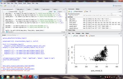
Fig. 1. RStudio software environment
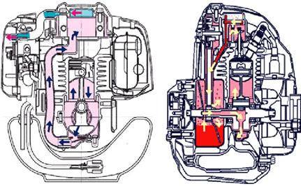
Fig. 2. Visualization of Honda GX25
motor

Fig. 3. Honda GX25
4. CONCLUSION
The application of the RStudio program in order to measure
data in terms of the diagnosis of internal combustion engines included
measurement data on the amplitude and speed of the Honda GX25 engine. This can
be expressed as a linear regression model in the following form:
![]() (14)
(14)
This equation enables the following interpretation:
the change of the parameter y on one
drive will change the value of the parameter X to 4.216. The parameter y in this case is the magnitude and
parameter X is the speed of the Honda GX25 engine, which is used in the Shell Eco-marathons.
Equation (14) is not the only outcome following application
of a linear model with two variables. This methodology also statistically
confirmed the fact that the model relating to (14) is based on the Ramsey
test, whose specifications were defined in the right form as errors. Meanwhile,
as this equation is able to include 98.9% of all measured values, it clearly calculates
the value of the coefficient of determination.
This
paper was elaborated within the framework of the following projects:
VEGA1/0197/14 – research on new methods and innovative design solutions in
order to increase efficiency and to reduce emissions of transport vehicle
driving units, together with the evaluation of possible operational risks; VEGA
1/0198/15 – research on innovative methods for emission reduction of driving
units used in transport vehicles and the optimization of active logistic
elements in material flows in order to increase their technical level and
reliability; and KEGA 021TUKE–4/2015 – development
of cognitive activities focused on innovations in educational programs in the discipline
of engineering branch, as well as building and modernizing specialized
laboratories specified for logistics and intra-operational transport.
References
1.
Hatrák
M. 2010. Ekonometria. [In Slovak: Econometrics]. Bratislava: IURA.
ISBN 978-80-8078-150-7.
2.
Piotrowski
J. 1995. Shaft alignment handbook. New
York: CRC Press.
ISBN 1-57444-721-1.
3.
Wackerly
D., W. Mendenhall, R. Scheaffer. 2008. Mathematical
Statistics with Applications. Belmont, USA: Thomson Brooks/Cole. ISBN-10:
0-495-38508-5.
Received 13.10.2015; accepted in revised form 02.03.2016
![]()
Scientific Journal of Silesian
University of Technology. Series Transport is licensed under a Creative
Commons Attribution 4.0 International License