Article citation info:
Kolarič, D., Kolarič, M. Example of flow modelling characteristics in diesel engine nozzle. Scientific Journal of Silesian University of Technology. Series Transport. 2016, 90, 123-135. ISSN: 0209-3324. DOI: 10.20858/sjsutst.2016.90.11.
Dušan KOLARIČ[1], Marko KOLARIČ[2]
EXAMPLE OF FLOW MODELLING CHARACTERISTICS IN DIESEL ENGINE NOZZLE
Summary. Modern transport is still based on
vehicles powered by internal combustion engines. Due to stricter ecological
requirements, the designers of engines are continually challenged to develop
more environmentally friendly engines with the same power and performance.
Unfortunately, there are not any significant novelties and innovations
available at present which could significantly change the current direction of
the development of this type of propulsion machines. That is why the existing
ones should be continually developed and improved or optimized their
performance. By optimizing, we tend to minimize fuel consumption and lower
exhaust emissions in order to meet the norms defined by standards (i.e.
Euro standards). Those propulsion engines are actually developed to such extent
that our current thinking will not be able to change their basic functionality,
but possible opportunities for improvement, especially the improvement of
individual components, could be introduced. The latter is possible by
computational fluid dynamics (CFD) which can relatively quickly and
inexpensively produce calculations prior to prototyping and implementation of
accurate measurements on the prototype. This is especially useful in early
stages of development or at optimization of dimensional small parts of the
object where the physical execution of measurements is impossible or very
difficult. With advances of computational fluid dynamics, the studies on the nozzles
and outlet channel injectors have been relieved. Recently, the observation
and better understanding of the flow in nozzles at large pressure and high
velocity is recently being possible. This is very important because the injection
process, especially the dispersion of jet fuel, is crucial for the combustion
process in the cylinder and consequently for the composition of exhaust gases.
And finally, the chemical composition of the fuel has a strong impact on the formation
of dangerous emissions, too. The research presents the influence of
various volume mesh types on flow characteristics inside a fuel injector
nozzle. Our work is based upon the creating of two meshes in the CFD software
package. Each of them was used two times. First, a time-dependent mass flow
rate was defined at the inlet region and pressure was defined at the outlet.
The same mesh was later used to perform a simulation with a defined needle lift
curve (and hereby the mesh movement) and inlet and outlet pressure. In next few
steps we investigated which approach offered better results and would thus be
most suitable for engineering usage.
Keywords: diesel engine, mass flow, CFD, needle
lift, injector, volume mesh
1. INTRODUCTION
The development of modern diesel
engines is directed to increase capacity and lower consumption. In future, it
will be especially oriented towards even greater fuel economy and purity of
diesel engines. Therefore, more and more manufacturers tend to develop engines
with smaller volumes, less cylinders and different systems for exhaust gas
treatment.
In achieving these goals, fuel
injection systems play an important role, since they are responsible for
just-in-time and regular supply of fuel to the engine cylinders. In the course
of time, there were several changes in their operation but the basic
characteristics remain the same until today. Increased awareness for the
environmental protection compel manufacturers to develop ever better and more
efficient fuel injection systems. The latest are electronically controlled and
allow precise control by opening and closing of valves, fuel injection time is
shorter while injection pressure is significantly higher. Electronically
controlled injection systems help to reduce harmful emissions (NOX,
soot) in the exhaust gases and to increase the engine power as well as reduce
the level of noise.
Such systems allow the injection
under high pressure (about 1500 to 2000 bars) which reduces the emissions of
solid particles. The higher the pressure, the better the dispersion (smaller
droplets) of the fuel is, which leads to better prepared mixtures at the same
time. By controlling the injection pressure that depend on the load and engine
frequency, these systems allow control of gaseous emissions and noise. For
simultaneous reduction of NOX and soot emissions, the optimal angle
of starting injection time is important. The latter is important due to the
interaction of different measures to reduce emissions of soot and NOX.
In turn, by reducing certain emissions, these measures often cause the increase
of others. The injection with common rail allows all the above requirements [1].
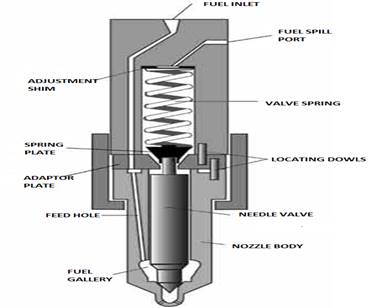
Fig. 1. Injector
The space, in which combustion takes
place, and the system of fuel supply are connected by the injector nozzle,
which is one of the most important elements of the fuel injection system. It is
used at the end of the compression phase to enable the supply of fuel under
high pressure to the combustion chamber. Injector nozzles take care of properly
atomized fuel, which is essential for good combustion, low fuel consumption and
the lowest emissions possible. Individual values of by-products of combustion
also depend on pressure of fuel injection, openness of nozzles and valves, fuel
characteristics and steering components [1].
Due to increased efficiency of the
process, several different versions of nozzles have been developed. Their
common task is to inject fuel into the cylinder of engine at optimum dispersion
[2].
2. DESCRIPTION OF EXPERIMENT
2.1. Computer fluid
dynamics (CFD)
Computers
have become an indispensable part of modern engineering practice. By using
computers, we can develop, design and improve old products faster. In the
sixties, the development of computer fluid dynamics has started. Its main
advantages, compared to conventional laboratory experiments, are the speed of
implementation, easy adaptability and lower price. Consequently, many
prototypes have not been required due to simulation which can figure out
whether something is going to work or not and can be improved by the use of
computer. For the purposes of CFD, there
are several different software packages. In our case, the program, which is
widely used in the automotive industry, was used for numerical simulation of
our problem. The program is based on the finite volume method to analyze fluid
flow [2].
2.2. Mathematical model of multiphase fluid flow in the selected CFD package
The object
of our research is the numerical analysis of simultaneous flow of two fluid phases
(vapor and liquid) through the injector of the fuel injection system. In order
to solve such a mathematical-physical model, it is necessary to solve a system
of conservation equations for each liquid phase separately.
The multiphase model describes each of the phases separately. The
conservation equations for each phase are connected with terms that describe
the transfer of mass, momentum, energy, turbulent kinetic energy and
dissipation of turbulent kinetic energy. These terms are the weakest point of
the multiphase model. In the Eulerian multiphase flow model, different
equations are separately numerically solved for each of the two phases (k and l) in the model [3].
Mass conservation:
![]() (1)
(1)
Here: rk – density of phase
k, ak – volume fraction
of phase k, vk – velocity of phase k, Gkl –
represents the interfacial mass exchange between phases k and l.
Here the
following condition must be fulfilled:
![]() (2)
(2)
Momentum conservation:
![]() (3)
(3)
Here: ![]() – body force vector which comprises gravity
– body force vector which comprises gravity ![]() and the inertial force in rotational frame,
and the inertial force in rotational frame, ![]() – pressure (values of pressure are supposed to
be equal for all phases),
– pressure (values of pressure are supposed to
be equal for all phases), ![]() – term which presents the momentum interfacial
interaction between phases k in l.
– term which presents the momentum interfacial
interaction between phases k in l.
The shear
stress ![]() of the k
phase is:
of the k
phase is:
![]() (4)
(4)
Reynolds
stress ![]() is:
is:
![]() (5)
(5)
Here: ![]() –
molecular viscosity,
–
molecular viscosity, ![]() – turbulent
viscosity
– turbulent
viscosity
Turbulent viscosity is modelled by:
![]() (6)
(6)
Energy (total enthalpy) conservation:
 (7)
(7)
Here: ![]() – heat (entalpy) source,
– heat (entalpy) source, ![]() – represents the exchange of enthalpy between
phases k and l;
– represents the exchange of enthalpy between
phases k and l; ![]() – enthalpy of phase k; qk – heat flux.
– enthalpy of phase k; qk – heat flux.
Heath
flux qk is defined
by:
![]() (8)
(8)
Here: ![]() –
thermal conductivity of phase k
–
thermal conductivity of phase k
Turbulent
heat flux![]() :
:
![]() (9)
(9)
Turbulent kinetic energy
conservation:
 (10)
(10)
The production term due to shear,
Pk, for phase k is:
![]() (11)
(11)
Turbulent dissipation equation: [4, 5]
 (12)
(12)
Specifying mass transfer (mass
interfacial exchange):
the linear cavitation model was used. It based on the following relation
for the mass exchange:
![]() (13)
(13)
Where: ![]() – mass
transfer, N''' – bubble number density, R – radius of bubbles.
– mass
transfer, N''' – bubble number density, R – radius of bubbles.
2.3. Data for
numerical calculation
Entry data for the calculation were obtained by measurements which were carried out in laboratory of engines on Friedmann & Maier device for testing outside vehicle injection systems. By using this device, data about the fuel mass flow and needle lift were collected and were used as boundary conditions in the simulation. They are presented in Figure 2.
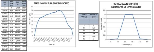
Fig. 2. Data about the fuel mass
flow (left) and needle movement (right)
The measurement was performed on the Bosch nozzle, type DLL 25 S 834, which is used in the engine of MAN D2566 MUM. The pressure of needle lift is 175 bars, the maximum lift of the needle is 0.3 mm. It has a bore diameter dn = 0.68 mm.

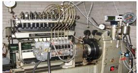
Fig. 3. Examined
injector (left) and Friedmann & Maier device for injection testing
systems (right)
2.4. Model mesh
The simulation was carried out on the geometric
model of the extreme lower part of the injector, which covers the tip of the
needle, seat area and bore for fuel injection (flow out channel). The
geometrical model was formed from the 2D structure in Figure 4 (left). For the
purpose of numerical simulations, there were created two spatial meshes on the
model, consisting of 250.000 (mesh 1) and 400.000 (mesh 2) elements. At each
mesh there were conducted two simulations: the one with defined mass flow and
the one with defined needle lift (Figure 4, right).
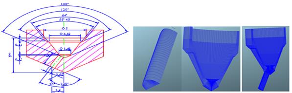
Fig. 4. Injector construction (left) and
model mesh (injector body, fuel injection bore,
combined in one body)
2.5. Boundary conditions of the model
The basic surfaces
(selections) of the model are: inlet, outlet and symmetry. For each of them
boundary conditions for multiphase flow were set. Furthermore, the parameters
for controlling the calculation, defining characteristics of the fuel, and
convergence criteria and parameters for postprocessing were determined.
In case of calculating the
defined needle movement, the type of simulation
"crank-angle" was used, which allows the change of conditions
depending on crank angle. Therefore, for the performance of these simulations,
besides the three already defined (Figure 5, left), 4 new selections were
created: Needle_move, Buffer, Interpolation and No_move (Figure 5, right).
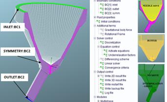
Fig. 5. Selections of boundary conditions
(left), operational tree, additional selections of boundary conditions in case
of defined needle movement (right)
3. ANALYZING RESEARCH RESULTS
The review of results
included the analysis of velocity, turbulent kinetic energy and volume fraction
in the outlet. Simulated values of the flow characteristics for both of the meshes
and for both approaches at the flow inlet and outlet are introduced below.
Examples illustrate the results after 0.001125 s of simulation (about half of
the process).
3.1. Velocity
The comparability of meshes
for both phases is relatively good in profile shape terms, but is very
different in absolute terms. As shown in the graphs, the calculated values for
the two phases are very similar at both the inlet and the outlet. However, the
difference between both approaches is substantial. The results match better at
the inlet to the bore. The values obtained with the defined needle movement
seem more realistic.
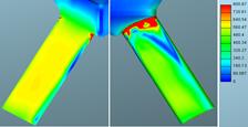
Fig. 6. Defined mass flow:
velocities of gaseous phase for mesh 1 (left) and mesh
2 (right) in m/s
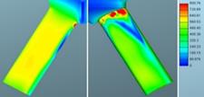
Fig. 7. Defined mass flow: velocities of
liquid phase for mesh 1 (left) and mesh
2 (right) in m/s
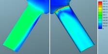
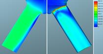
Fig. 8. Defined
needle lift: velocities of gaseous phase for mesh 1 (left) and mesh
2 (right) in m/s
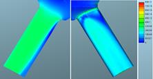
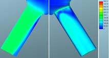
Fig. 9. Defined needle lift: velocities of liquid phase for mesh 1 (left) and
mesh
2 (right) in m/s
Fig. 10. Comparison of velocity profiles:
Gaseous phase (left) – defined mass flow for meshes 1 and 2 and the defined
needle lift for meshes 1 and 2; Liquid phase (right) – defined mass flow for
meshes 1 and 2 and the defined needle lift for meshes 1 and 2
3.2. Turbulence
kinetic energy
The comparison of results
between the two meshes shows that the results of TKE are relatively well
matched, and that there are only noticeable differences along the walls, while
after that the flows subside. Slightly larger deviation is observed in the
gaseous phase at the exit of the hole which is confirmed by the graphs of
numerical values. The mesh density seems to have made a large impact on both
approaches.
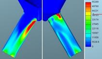
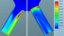
Fig. 11. Defined mass flow: Turbulence
kinetic energy of gaseous phase for mesh 1 (left)
and mesh 2 (right) in m2/s2
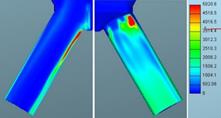
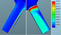
Fig. 12. Defined mass flow: Turbulence
kinetic energy of liquid phase for mesh 1 (left)
and mesh 2 (right) in m2/s2
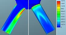
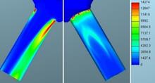
Fig. 13. Defined needle lift: Turbulence
kinetic energy of gaseous phase for mesh 1 (left)
and mesh 2 (right) in m2/s2
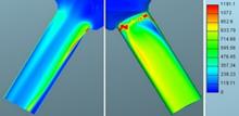
Fig. 14. Defined needle lift: Turbulence
kinetic energy of liquid phase for mesh 1 (left)
and mesh 2 (right) in m2/s2
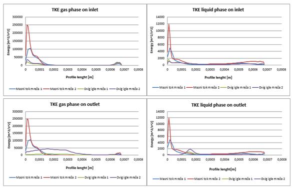
Fig. 15. The
comparison of Turbulence kinetic energy (defined mass flow and needle lift -
meshes 1 and 2)
3.3. Volume fraction
The volume fractions match well
at the inlet, but some differences can be observed at the outlet of the bore.
This means that the gaseous phase moved closer to the center of the bore.
100% of gaseous phase![]()
![]()
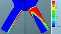
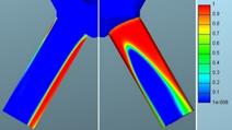
Fig. 16. Defined mass flow: Volume fraction of
gaseous phase for mesh 1 (left)
and mesh 2 (right)
100% of gaseous phase![]()
![]()
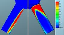
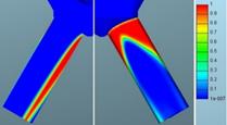
Fig. 17. Defined needle lift: Volume fraction of
gaseous phase for for mesh 1 (left)
and mesh 2 (right)
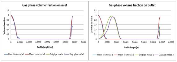
Fig. 18. The comparison of volume fraction
(defined mass flow and needle lift)
for meshes 1 and 2
4. CONCLUSIONS
In
the field of computational fluid dynamics, there is still quite a lot of
potential for improvement and innovation. Therefore, our research presents two
different modes of injector nozzle simulation and we try to determine whether
they are comparable or not. The first approach dealt with the defined
time-dependent mass flow at the entrance to the injector, and the data were
obtained experimentally. In the second case, the modelled calculations were
replicated with the defined needle lift and the pressure at the inlet. Both
were used at two different mesh volumes of numerical model.
It turned
out that the approaches gave different results. The particularly large
deviations occured in the calculated values of pressure and velocity. Much more
comparable results were gained by turbulent kinetic energy and volume
fractions.
It was also
noted that the discrepancy was greater at the exit of the bore. In both
approaches, partial reasons for the deviations resulted from in the inability
of choice of exactly the same time interval, although measurement error was
also possible. However, those factors could not be the cause of such large
deviations in the case of pressure, especially because in the post-analysis,
the possibility of incorrect settings in the control file was excluded.
Nevertheless,
we managed to approximate the results in two ways. First, the inlet pressures
were taken out of the results of simulation which was using the approach with
the defined mass flow. This information was then set as a boundary condition in
simulation, in which we defined the needle lift and pressure at the inlet. The
match was much better. Therefore, we believed that with some adjustments of
incoming data, especially with more accurately defined mass flow, we could
achieve a very good match. Then we did the reverse, and from the simulation
with the defined needle lift, the mass flows were received and were determined
at the inlet. There was again a very good match in results.
Despite
that, in the initial research phase, we could not confirm whether the approach
was entirely comparable or not. We estimated that it would make sense to re-do
the measurement of mass flow and needle lift, and after that simulations should
be replicated with much more accurate mathematical analysis of physical
conditions of the process, which would be subject to further consideration of
the problem.
References
1.
Kegl B. 2006. Osnove motorjev z notranjim zgorevanjem.
[In Slovenien: Fundamentals
of internal combustion engines]. Maribor: Fakulteta za strojništvo.
2. Volmajer M. 2001.
„Numerična in eksperimentalna analiza tokovnih karakteristik vbrizgalne šobe
dizelskega motorja”. [In Slovenien: “Numerical and experimental analysis of
flow characte9ristics of the injectors for diesel engines”]. MSc thesis. Maribor: TF.
3. Volmajer M. 2007. “Modeliranja večfaznih tokov v
vbrizgalni šobi”. [In Slovenian: “Modeling of multiphase flows in the injector”].
PhD thesis. Maribor: TF.
4. Manual Fire. AVL List GmbH. 2011. Graz.
5. Turbulence
modeling for beginners. Tennessee: Tony
Saad, University of Tennessee Space Institute. 2014. Available at:
http://www.cfdonline.com/W/images/3/31/Turbulence_Modeling_For_Beginners.pdf.
Received 11.08.2015;
accepted in revised form 21.12.2015
![]()
Scientific Journal of Silesian
University of Technology. Series Transport is licensed under a Creative
Commons Attribution 4.0 International License