Article
citation information:
Illes, L., Jurkovic, M., Kalina,
T., Gorzelanczyk, P., Luptak, V. Methodology for optimising the hull shape of a vessel
with restricted draft. Scientific Journal
of Silesian University of Technology. Series Transport. 2021, 110, 59-71. ISSN: 0209-3324. DOI: https://doi.org/10.20858/sjsutst.2021.110.5.
Ladislav ILLES[1],
Martin JURKOVIC[2],
Tomas KALINA[3],
Piotr GORZELANCZYK[4],
Vladimir LUPTAK[5]
METHODOLOGY
FOR OPTIMISING THE HULL SHAPE OF A VESSEL WITH RESTRICTED DRAFT
Summary. Increasing transport
volumes on Europe's inland waterways is a major reason for improving the
quality and reliability of internationally important waterways. Continued
navigation restrictions due to restricted draft (draught) led to the search for
new design solutions. Such solutions enable navigation even under critical
navigation conditions. Restricted draft is one of the most important
limitations that hinder navigation, especially in the summer. The main
objective of the construction of an inland vessel is to obtain a shape that
will achieve optimum performance with as little resistance as possible. A shape
that will be able to navigate at a limited depth. Presently, there is no
clearly defined methodology as a procedure for optimising the hull. When
solving theoretical problems of shipbuilding character and ship calculations,
it is necessary to consider the basic theory of the ship with special regard to
the latest methodological procedures of related scientific disciplines. This
paper presents a methodology that considers all the basic aspects of
optimisation tasks in ship design and construction.
Keywords: optimisation, methodology, restricted draft,
waterways, vessel
1. INTRODUCTION
Shipping on
European rivers and inland waterways is of considerable economic benefit,
contributing to the carriage of goods and passenger transport. The most
important waterway is the Rhine-Main-Danube Canal, which connects the North Sea
with the Black Sea. However, shipping on some significant critical stretches of
the Danube has been restricted by long-standing problems of limited seasonal
navigation conditions. Sometimes the traffic of large commercial vessels and
pushed convoys is completely paralysed [9,11].
The flow
regime and water level has been developing and changing globally for a long
time. This is due to anthropogenic effects such as water management operation
or land use change near waterways. This has an impact on freshwater resources
and changes in hydrological conditions that form the basis for water resources
and the entire ecosystem [5].
Because of
rapid climate change in recent years, there have been serious seasonal problems
on the Rhine, where it has become necessary to restrict freight transport to
such an extent that it has caused difficulties in the logistics systems of
large companies that mainly source their raw materials and semi-finished
products through shipping [2]. These changes represent a global problem for navigation
on inland waterways, water areas and ports and have become major obstacles to
the further development of water transport [16,19].
Traffic
restrictions due to the low water level can similarly be seen on the Danube
River. In January 2017, the water levels were extremely low, around the lowest
navigable water level (LNWL), when the river froze over, and subsequently, ice
events occurred. Ship traffic on the Upper Danube and the Middle Danube saw a
considerable decline in loaded drafts during this period. After measures to
combat the ice events on the Danube had been concluded and navigation
conditions stabilised, operation at loaded drafts of approx. 2,5 m for barges
in pushed convoys began in early March. Hydrological conditions on the Danube
were unstable during the second quarter, and by late May, loaded drafts were no
more than 2,3-2,2 m. [4]. The summer low-water period began in June, and
successive, intermittent precipitation in the third and fourth quarters did not
lead to a stabilisation of hydrological conditions, hence, loaded drafts
remained between 2, 2 and 2, 3 m from September until the end of the year 2017
[3].
The low water
level lasted for 80 days, resulting in the cessation of navigation and the
associated losses for shipowners [1]. Optimising the shape of the vessel's hull
is one way to improve shipping operations on inland waterways. Particularly,
the improvement of the navigability characteristics of vessels navigating in
shallow waters. Restricted draft is one of the most important limitations that
reduces navigation, especially during summer.
An inland
vessel floating in shallow water achieves a much higher resistance than a
vessel floating in deep water. There are several methods by which these effects
can be eliminated [8,15,21,25,27]. In addition to resistance, wake fraction and
thrust deduction change as well [20,23]. The propulsion efficiency likewise
varies depending on the different propeller load [12]. Optimisation of ship
hull–propeller system is also one of the most important aspects of ship
design and leads to ship cost reduction, improving performance and increasing
the lifespan of the propulsion system. Changes in the stream of water
surrounding the vessel are caused by different flow around the hull compared to
deep water navigation [7]. The low ship underneath below the vessel leads to
increased return flow speed. In the vertical direction, the movement of water
is limited, causing it to be transformed into a horizontal movement. Thus, the
increased reverse flow rate reduces the pressure below and around the hull.
This results in an additional reduction in the draft and, in most cases,
increased wave resistance [13,26].
The specific
effects that change the trajectory of liquid flow around the ship hull in
shallow water require different design requirements compared to seagoing ships.
Inland vessels often navigate in waters with a depth of about 2 m. The main
objective of the design of shallow-water vessels is to achieve the shape of the
hull, with the lowest propulsion power requirements. Navigation optimisation
studies, focusing on the impact of waves on shallow watercraft, have been
conducted in the past [22,24,29].
This paper is
based on the objectives set out in the Danube Strategy and follows up the
scientific publications on the research and development of new and innovative
types of ships and propulsion vehicles designed for the changing conditions of
the Danube navigation. However, the results are general, globally applicable on
inland waterways with similar parameters. The result of this paper is a
methodology of optimising the shape of the ship hull with restricted draft,
which will be the basis for the application part with a specific proposal of
solution.
2. THEORETICAL
BACKGROUND AND METHODS
In
solving the theoretical problems of shipbuilding character and naval
architectural calculations, the basic theory of ship will be applied with
special regard to the latest published results of related scientific
disciplines.
2.1.
Equations describing fluid flow
When
examining fluid flow, the basic laws of physics apply, that is, conservation
law of mass, conservation law of momentum and conservation law of energy. All
these laws, as well as viscous phenomena in real fluid, are reflected in
Navier-Stokes equations that describe both laminar and turbulent flow.
For
incompressible fluids, where ρ = const., and ![]() , the
continuity equation in a
differential form will be:
, the
continuity equation in a
differential form will be:
![]() (1)
(1)
When
a hexahedron represents the liquid particle, its centre of gravity will be
affected by the mass forces X, Y and Z in the corresponding
directions. Surface forces from external pressure will act in the centre of
gravity of the elementary body surfaces.
The
hydrostatic Euler equations in the state of flow will have nonzero values on
the right side. These will be x, y, and z acceleration components
that express forces per unit mass.
Hydrodynamic
Euler equations for the ideal fluid (when viscosity is not considered) are then
obtained by substituting the inertia forces generated by the acceleration of
the fluid particles into the equations:
![]()
![]() (2)
(2)
![]()
whereby
adjusting the accelerations on the right side, we get Euler's partial
differential equations that express the dependence between unit mass, surface
and inertia forces:
![]()
![]() (3)
(3)
![]()
Derivatives
according to x, y and z on the right side of the equations
express the acceleration components along the curved streams. The last
derivative by t is a local component that expresses the change in
velocity over time.
Considering
both the flow viscosity of the fluid, and the corresponding shear forces would
also act on the walls of the elemental hexahedron - in addition to the
compressive forces.
Newton’s
equation expresses these frictional forces mathematically as tangential stress
![]() (4)
(4)
where η
is the coefficient of dynamic viscosity.
By
adding the friction component to the Euler equations of fluid dynamics, we
obtain the Navier-Stokes partial differential equations for all unit actions on
the fluid particle in three basic directions of space, that is, weight,
pressure, friction and inertia. Furthermore, considering the continuity
equation (1), the Navier-Stokes equations expressing the flow of Newtonian
fluid can be further simplified to the form:
![]()
![]() (5)
(5)
![]()
Equations
5 can be interpreted as the specific form of the second Newton's law for the
flow of viscous incompressible fluid per unit mass, on the right with the
product of acceleration and weight, on the left with the sum of mass and
surface (pressure and viscous) forces [6,10].
2.2.
Computational domain and CFD mesh
Computational
Fluid Dynamics (CFD) is the most commonly used software in computer modelling
of fluid flow. Several mesh-based methods have been developed in this area
where the geometry under investigation is replaced by a 2D or 3D mesh and the
flow problem is solved using Navier-Stokes equations. The basic principle of
CFD is to create a computational domain that consists of a geometric model of
the actual and discretised form (mesh), a definition of boundary conditions, a
set of physical properties and calculation methods, and possibly external
geometry boundaries of the flow area (external flow) [17,28].
In
the CFD simulation of navigation, the geometry under investigation consists of
the outer surface of the hull, surrounded by a flow area, mostly of hexahedral
shape. This is a typical case of external flow where the flow takes place in
the surrounding environment and not within the computational geometry. The
investigated physical phenomena take place in a multiphase environment, at the
boundary of two phases (water-air), which considerably increases the
computational complexity of these tasks.
The
resulting mesh is a product of discretisation of real geometry, its arrangement
can be either structured or unstructured.
Structured
mesh consists of rectangular elements (in 2D) and hexahedral blocks (in 3D).
The main advantage of such a mesh is higher accuracy of calculation and less
complex matrix representation of the solved structure within the algorithm.
However, the discretisation of complicated shapes and the creation of
transition areas with different meshing size often give rise to problems that
point to less flexibility in the structured mesh.
In
some cases, an unstructured mesh with sufficient accuracy can be similarly
used. More so, there are tasks that do not allow the application of structured
meshes. Such a mesh consists of triangular elements (in 2D) or tetrahedral,
prismatic pentahedron and pyramidal elements (in 3D). It is ideal for
discretising complex geometric shapes, maintaining good quality in shape
interpolation (small distortions), and densifies without problems. The various
elements are often combined into an optimal structure, for example, in the
boundary layer zone.
Another
possibility is the creation of hybrid structures, which is a suitable
combination of structured and unstructured meshes. It has wide application in
CFD simulations, where the complex surfaces of bodies and their boundary layers
are represented by an unstructured mesh, while the environment is formed by a
high-quality structured mesh. The interface zone between them is a transition
area filled with pyramidal elements (in 3D).
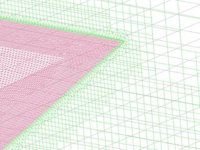
Fig. 1.
Structured (right) and unstructured (left) mesh with boundary layer and
intermediate zone connected to the refined structured mesh
The most serious limitation in CFD analysis is the
number of mesh elements and nodes. In each iteration of the calculation,
the hydrodynamic state of the elements is evaluated individually, and their
excessive number can massively increase computational complexity and machine
time. Hence, it is necessary to keep the number of elements as low as possible,
however, not to the detriment of the accuracy of the calculation.
We call a quality mesh when the elements have the
same size, are geometrically regular and their distribution is also regular in
the discretised area. A suitable choice of element size ensures that the
hydrodynamic properties of the flow are captured; however, velocities are
decisive for dimensions.
In most cases, due to the limited number of
elements, it is not possible to capture the effects in different areas of a
domain while meeting all mesh quality criteria. This problem is solved by local
refinement of the mesh in computationally demanding and geometrically complex
parts of the model. Typical examples are the boundary layer region, leading and
trailing edges, free fluid surfaces, etc.
In terms of the motion state of the investigated
solids at the boundaries of the computational domain, individual areas of the
mesh can be stationary, deformable and dynamic. Generally, dynamic meshes can
be used wherever the domain shape changes over time due to the rotational or
translational movement of its boundary surfaces. During the simulation, the
dynamic mesh and the surrounding mesh zone must be continuously smoothed and
remeshed, placing increased demands on computing power [6,10].
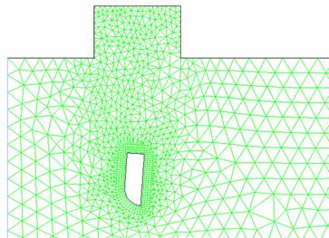
Fig.
2. Dynamic mesh zone around a falling body in a 2D CFD simulation
(ANSYS
Fluent 17.2 Documentation)
2.3.
Methods for solving partial differential equations (PDE) of CFD
Many
numerical methods have been developed to address particular physical problems.
Their application depends both on the suitability of the method for solving the
issue and on the history of development.
By
replacing the geometry of the examined area with a mesh of generated nodal
points, the flow calculation domain is discretised, thus, allowing the flow
equations to be converted into algebraic equations.
Solutions
of differential and integral flow equations by discretisation are carried out
through various methods, of which the following are the most common:
Finite
Volume Method (FVM) - This method in a discretised form retains very reliably,
the principles of conservation laws of balanced physical quantities in the
control volume and is, therefore, the most widely used CFD simulation apparatus
for solving the Navier-Stokes equations.
Finite
Difference Method (FDM) - This method is based on the conservative differential
form of determining equations. It is a traditional and proven method for
numerical solution of partial differential equations. The principle of this
method is to transform derivatives into differences in the mesh nodes of the
flow field.
Finite
Element Method (FEM) - This method uses elements instead of control volumes.
Balancing laws are applied to the elements to determine the quantities of the
flow field at the nodes of the elements. Unlike the previous two methods, this
method also uses interpolation structures to ensure the interdependence of
nodal points.
For
the solution of algebraic equations, an optimal algorithm (scheme) of the
solution is provided, which is the basis for computer software development.
Schemes specify iterative processes and may be explicit or implicit. The
practical solution is performed using a software and the process should
gradually converge to an exact solution. The aim is to achieve a minimum
deviation from the exact result.
The
best-known solution schemes applied in the CFD area are Euler FTFS scheme,
Euler FTCS scheme, Euler FTBS scheme, Upwind scheme, Lax-Friedrichs scheme,
Lax-Wendroff scheme, MacCormack scheme, Runge-Kutta scheme. [18].
2.4.
Models for turbulent fluid flow
Numerical
modelling of turbulent flows is still in the process of research and
development, supported by the latest knowledge of mathematics, physics and
technical computational methods. However, there is no universal model of
turbulence that is generally and effectively applied in all cases. To choose the
most suitable model for a particular calculation case, it is necessary to
consider the possibilities and limitations of individual numerical models.
Turbulent swirls are characterised by length and speed scales and the following
methods are appropriate for different scales:
Direct
Numerical Simulation (DNS) - This method is suitable for direct solution of a
wide range of turbulent vortex sizes, based on Navier-Stokes equations. It does
not model swirls but captures turbulence by solving equations with high
precision, which requires a very fine mesh. Direct numerical simulation
provides a perfect mapping of physical phenomena in a flowing fluid, and its
results are considered equivalent to those of experiments. Many mesh elements
and a time-dependent process with very small steps lead to the technical
unrealisability of simulations in engineering practice.
Large
Eddy Simulation (LES) - This method solves only large-scale swirls that can be
captured by a coarse mesh at larger time steps. For small turbulent swirls,
subgrid models are created and removed by filtration of the turbulent field.
Their right combination allows creating a coarse mesh even in engineering tasks
whose solution is already realistic with today’s computer technology.
However, a major disadvantage of the large vortex method is the need to refine
the mesh along the body walls in three directions. Various modified methods as
well as a RANS/LES hybrid model have been developed to overcome this drawback.
Time-Averaging
Method (RANS - Reynolds Averaged Navier-Stokes Equations) - This method has
relatively low computational capacity requirements and provides acceptable
accuracy. It is being extensively used in engineering simulations. Further, it
consists of parametric modelling of turbulent flow by time-averaged values of
physical quantities using Reynolds method. Several different RANS methods have
been developed for various specific task types, which simplify the modelling of
swirls using added transport equations. There is also a method known as DES
(Detached Eddy Simulation) which is a transition between RANS and LES. It
combines the advantages of both the LES and the RANS numerical modelling
methods.
Some
of the time-averaging methods are based on Reynolds stresses (RSM), others are
based on the Boussinesque hypothesis of turbulent viscosity (for example, k - 𝜀
and 𝑘 - 𝜔).
Results calculated by RANS should be confronted with published results or
validated by experiment. The most common models of turbulence based on Reynolds
averaging and Boussinesque principle, which are also implemented by ANSYS
Fluent program are:Spalart-Allmaras Model, 𝑘 - 𝜀
Models, 𝑘 - 𝜔
Models, 𝑘 - 𝑘𝑙 - 𝜔
Transition Model, Transition SST Model, Reynolds Stress Model (RSM), Large Eddy
Simulation (LES) Models, Wall Adapting Local by Eddy Viscosity (WALE) Model,
Detached Eddy Simulation, Smagorinsky Lilly Models, Dynamic Kinetic Energy
Subgrid Scale Model, Scale-Adaptive Simulation (SAS) Model.
The
appropriate optimisation method must be chosen and the specific optimisation
task will be formulated only after the precise determination of the maximised
and minimised variables (ship parameters) and limiting conditions (waterway
restrictions, economic objectives, etc.). A volume of results of technical
analyses and the way of their processing also have a major impact [14].
3. RESULTS AND
DISCUSSION
Creation of a
three-dimensional CFD domain for the analysis of navigational characteristics
of vessels is usually started in some solid or surface modelling program.
A solid block with a cavity corresponding to
the negative shape of the hull is created. The flow-around is being
investigated; this is a typical problem of external flow in CFD. Only one half
of the space is modelled because in these cases the boundary condition of symmetry
can be applied in the ship's centre plane (XZ). Such a typical 3D model is
shown in Figure 3, this particular domain was created for a pontoon-type
single-hull test.
Thereafter, after importing the 3D
model into the CFD system, the three-dimensional domain body is replaced with a
suitable task-specific computational mesh. The mesh is refined in critical
areas, special elements are created in the boundary layer and the transition
areas. Figure 4 is an overall view of the computational grid, showing that the
grid is refined around the body to be flown around and in the free surface area
to better capture the physical effects such as turbulence, streamline
separation and wave motion.
A cross-sectional view of Figure 5
provides a more detailed insight into the internal structure of such a CFD
mesh. It is possible to distinguish individual special types of elements -
prismatic in the boundary layer, pyramidal in the transition area and
structured surroundings formed by hexahedral elements of different sizes.
After
successfully creating the required quality mesh, the computational domain is
configured based on input parameters and specifically for the type of analysis.
When the system is properly configured, the transient analysis is started, only
then the convergence of the calculation is monitored until termination.

Fig.
3. Example of initial 3D model of a CFD domain intended for
vessel flow-around simulation
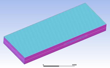
Fig.
4. Computational mesh of CFD domain with refined zones
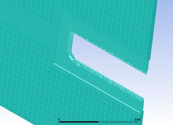
Fig.
5. Internal structure of 3D mesh with different zones
Figure
6 shows the resulting wave field of the vessel. It is an example of CFD
analysis of the hull where the physical properties of the flow-around were
investigated. In addition, the resistance of the hull was determined at certain
constant cruise speeds. It is very important to compare these analysis results
with proven technical indicators of other vessels that have been previously
model-tested. In most cases, this is an adequate result validation method. By
gradual calibration of the CFD task configuration, such as dimensions and
proportions of the computational domain, mesh parameters, boundary layer,
boundary conditions, initialisation parameters, computational model and
numerical methods, it is possible to refine the result and achieve accuracy
with a deviation of ± 5%. Such deviations from the results of other
sources are satisfactory and the accuracy of CFD analysis is sufficient to
perform optimisation tasks.
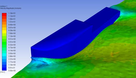
Fig. 6.
Example output from CFD analysis of flow-around a vessel – wave pattern
The emergence of the question, what is new in the
mentioned methodology, comes to bear at the end of this study. Similar
progressive approaches have been applied for several years in various companies
and institutions specialised in hydrodynamic development and research.
Here, however, it is a question of finding new ways,
for example, researching new principles of hull interaction with multiple
propulsion units, determining their optimal number, thrust and location. Of
course, such innovation requires major changes in the shape of the hull and in
the hydrodynamic parameters of the flow-around. Due to the distribution of
propulsion power to several propulsion units over the entire length of the hull
and the low draft, the introduction of new types of special propulsors should
be considered as well. It is possible to analyse their properties as a single
unit submerged in a basin by CFD analysis.
More important is the simulation of their
interaction with the hull, which is a much more complex problem due to their
increased number and the special hydrodynamically shaped underwater part of the
hull. The classic single-propeller and twin-propeller arrangement is presently
well documented, and the velocity field influenced by the hull flow-around in
the plane of the propeller can be illustrated by the standard wake field
diagram. However, current science still has debts in the complex theory of
distributed propulsion and their interaction with the hull for cases where some
units have to work in the flow field of others, that is, their velocity fields
interact.
This is a rather complex issue that the R&D has
been trying to resolve in the past by model tests when full functional
propulsion units have been mounted on models, scaled in proportions given by
the theory of similarity. However, these tests are very time-consuming and
costly; therefore, are not appropriate at the research stage or for extensive
optimisation processes. Therefore, in recent years, such CFD simulations have
already begun, which have already considered the effect of the propulsors on
the flow-around and the total flow field nearby the hull. Manufacturers of
commercial CFD software have developed tools that allow defining constant flow
velocities at several selected locations of the computational domain, and in
this way, simulate the operation of the propulsors in a simplified way.
Rotating dynamic meshes that can represent the body
shape of the propulsor and its surroundings are available for better accurate
analysis. This means that within one domain we can have 3D models of the hull
and all propulsors, combining static and dynamic meshes. Of course, this method
is computationally demanding, however, it is already practically applicable
with the current computer technology.
4.
CONCLUSION
The methodological process is designed to solve complex shipbuilding
tasks and partial optimisation tasks. Among the basic tasks are, for example,
the design and analysis of the characteristics of the new shapes of the ship's
displacement hulls, considering the long-term proven hulls of inland waterway
vessels.
Another area of application of the methodology is the sizing of the new
arrangements on the session: hull - propulsion, considering long-established
inland navigation systems. Application of the results can similarly be
practised in CFD analysis and comparison of performance parameters of new
conceptual and existing solutions.
This methodology is designed to achieve other specific solutions:
· the development of an
innovative concept for a new generation of inland waterway vessels,
· simple identification of
optimal main ship parameters based on input data, such as navigational
restrictions and economic targets,
· support tools or working
aids for ship planners, such as the implementation of the proposed methodology,
· preliminary input for
economic calculations of shipping establishment and operating costs.
Due to the lower overall complexity, the CFD method
has wide application, which in this particular investigation, is the only real
alternative for optimisation of distributed propulsion. This is just one of the
possible directions for further development of low-draft ships. The ultimate
goal is to put an entirely new, innovative type of inland vessel into service
in the foreseeable future.
References
1.
90th Session of the Danube Commission.
2018. Market observation for Danube
navigation - results in 2017.
Budapest. Danube Commission.
2.
Aguiar F-C., J. Bentz, J-M.N. Silva, A-L. Fonseca, R.
Swart, F-D. Santos,
G. Penha-Lopes. 2018. “Adaptation to climate change at local level in
Europe: An overview”. Environmental
Science & Policy 86: 38-63. ISSN: 1462-9011. DOI: https://doi.org/10.1016/j.envsci.2018.04.010.
3.
Beuthe M., B. Jourquin, N. Urbain, I. Lingemann, B.
Ubbels. 2014. “Climate change impacts on transport on the Rhine and
Danube: A multimodal approach”. Transportation
Research Part D: Transport and Environment 27: 6-11. DOI: https://doi.org/10.1016/j.trd.2013.11.002.
4.
David A., E. Madudova. 2019. “The Danube river
and its importance on the Danube countries in cargo transport”. 13th International Scientific Conference on
Sustainable, Modern and Safe Transport, “TRANSCOM 2019” 40:
1010-1016. 29-31 May 2019. Novy Smokovec, Slovakia.
5.
Doll P., B. Jimenez-Cisneros, T. Oki, N.W.
Arnell, G. Benito, J.G. Cogley, T. Jiang, Z.W. Kundzewicz, S. Mwakalila, A.
Nishijima. 2014. „Integrating risks of climate change into water
management”. Hydrol. Sci. J.
60: 4-13. DOI: 0.1080/02626667.2014.967250.
6.
Douglas J.F., J.M. Gasiorek, J.A. Swaffield, L.B.
Jack. 2005. Fluid mechanics.
Fifth edition, Pearson Education Limited, Harlow. ISBN: 978-0-13-129293-2.
7.
Esmailian E., H. Ghassemi, H. Zakerdoost. 2017.
“Systematic probabilistic design methodology for simultaneously
optimizing the ship hull - propeller system”. International Journal of Naval Architecture and Ocean Engineering
9(3): 246-255. ISSN: 2092-6782. DOI: https://doi.org/10.1016/j.ijnaoe.2016.06.007.
8.
Ferreiro L.D. 1992. “The effects of confined
water operations on ship performance: a guide for the perplexed”. Nav. Eng. J. 104: 69-83.
9.
Galierikova A., J. Sosedova. 2018. “Intermodal
Transportation of Dangerous Goods”. Nase
More 65(3): 8-11. ISSN: 0469-6255. DOI: 10.17818/NM/2018/3.8.
10.
Ganco M. 1983. Fluid
mechanics. Bratislava: ALFA Bratislava. ISBN: 63-745-83.
11.
Habersack H., T. Hein, A. Stanica, I. Liska, R. Mair,
E. Jager, Ch. Hauer, Ch. Bradley. 2016. “Challenges of river basin
management: Current status of, and prospects for, the River Danube from a
river engineering perspective”. Science
of The Total Environment 543(A): 828-845. DOI:
https://doi.org/10.1016/j.scitotenv.2015.10.123.
12.
Harvald S.A. 1977. “Wake and thrust deduction at
extreme propeller loadings for a ship running in shallow water.” RINA Suppl. Pap. 119.
13.
Kim D.H., J.K. Paik. 2017. “Ultimate limit
state-based multi-objective optimum design technology for hull structural
scantlings of merchant cargo ships”. Ocean
Engineering 129: 318-334. ISSN: 0029-8018. DOI: https://doi.org/10.1016/j.oceaneng.2016.11.033.
14.
Kudelas D. 2017. Basics of computer flow modelling
and visualization. Kosice: Faculty
BERG TU, Kosice.
15.
Lackenby H. 1963. “The effect of shallow water
on ship speed”. Shipbuild. Mar. Eng. 70: 446-450.
16.
Lobanova A., S. Liersch, J.P. Nunes, I. Didovets, J.
Stagl, S. Huang, H. Koch, M.R.R. Lopez, C.F. Maule, F. Hattermann, V.
Krysanova. 2018. “Hydrological impacts of moderate and high-end climate
change across European river basins”. Journal
of Hydrology: Regional Studies 18: 15-30. ISSN: 2214-5818. DOI: https://doi.org/10.1016/j.ejrh.2018.05.003.
17.
Macháčková A., P. Kuchta, Z.
Klečková, R. Kocich, J. Szwed. 2016. “Numerical simulation of
the heat treatment of the weld for steam generator”. Metalurgija 55(4): 741-744.
18.
Molnar V. 2011. Computational
Fluid Dynamics - Interdisciplinary Approach with CFD. Bratislava: STU
Bratislava. ISBN: 978-80-8106-048-9.
19.
Nouasse H., A. Doniec, G. Lozenguez, E. Duviella, P.
Chiron, B. Archimede, K. Chuquet. 2016. “Constraint satisfaction
problem based on flow graph to study the resilience of inland navigation
networks in a climate change context”.
IFAC-PapersOnLine 49: 331-336. DOI:
https://doi.org/10.1016/j.ifacol.2016.07.626.
20.
Raven H. 2012. “A computational study of
shallow-water effects on ship viscous resistance”. Proceedings of the 29th Symposium on Naval Hydrodynamics.
Gothenburg.
21.
Raven, H. 2016. “A new correction procedure for
shallow-water effects in ship speed trials”. Proceedings of the 2016 PRADS Conference, Copenhagen.
22.
Rotteveeel E., R. Hekkenberg, A. Ploeg. 2017.
“Inland ship stern optimization in shallow water”. Ocean Engineering 141: 555-569. ISSN:
0029-8018.
23.
Rotteveel E., R. Hekkenberg. 2015. “The
influence of shallow water and hull form variations on inland ship
resistance”. Proceedings of the
12th International Marine Design Conference. “IMDC 2015”. 11-14 May 2015. Tokyo, Japan.
24.
Saha G.K., K. Suzuki, H. Kai. 2004.
“Hydrodynamic optimization of ship hull forms in shallow water”. J. Mar. Sci. Technol 9: 51-62. DOI:
10.1007/s00773-003-0173-3.
25.
Schlichting O. 1934. Ship's resistance to limited water depth: Resistance of ships to
shallow water. Jahrb. der Schiffbautech 35: 127.
26.
Sun H., O.M. Faltinsen. 2012. “Hydrodynamic
forces on a semi-displacement ship at high speed”. Applied Ocean Research 34: 68-77. ISSN: 0141-1187. DOI:
https://doi.org/10.1016/j.apor.2011.10.001.
27.
Tuck E. 1978. “Hydrodynamic
problems of ships in restricted waters”.
Annu. Rev. Fluid Mech 10: 33-46. DOI:
10.1146/annurev.fl.10.010178.000341.
28.
Wang X.M., X.L. Wu, W.Q. Zhou. 2019. “Analysis
of oxygen enriched combustion characteristic of 350 MW utility boiler based on
computational fluid dynamics”. Metalurgija
58(3-4): 223-227.
29.
Zhao L-e. 1984. “Optimal ship forms for minimum
total resistance in shallow water”. Schr.
Schiffbau. DOI: 0.15480/882.930.
Received 04.07.2020; accepted in revised form 19.10.2020
![]()
Scientific
Journal of Silesian University of Technology. Series Transport is licensed
under a Creative Commons Attribution 4.0 International License