Article
citation information:
Marinov, M., Petrov, Z. A static calibration of MEMS 3-axis
accelerometer using a genetic algorithm. Scientific
Journal of Silesian University of Technology. Series Transport. 2019, 105, 157-168. ISSN: 0209-3324. DOI: https://doi.org/10.20858/sjsutst.2019.105.13.
Marin MARINOV[1],
Zhivo PETROV[2]
A STATIC CALIBRATION OF
MEMS 3-AXIS ACCELEROMETER USING A GENETIC ALGORITHM
Summary. In this paper, a procedure for MEMS accelerometer
static calibration using a genetic algorithm, considering non-orthogonality was
presented. The results of simulations and real accelerometer calibration are
obtained showing high accuracy of parameters estimation.
Keywords: MEMS accelerometers,
calibration, bias, genetic algorithm
1. INTRODUCTION
Various microelectromechanical
systems (MEMS) are used in different devices. Some of the most used are MEMS
accelerometers. There are many areas of MEMS accelerometers application, such
as location of objects, tracking of human movement, control of mirrors in
cameras, etc. [2,3,5,11]. They are small, lightweight
and provide digital outputs, but possess relatively large errors. Different
ways of accelerometer calibration are used to improve accuracy.
The most important step for
accuracy improvement is the static calibration of the accelerometer. It must be
done separately for each particular accelerometer. There are two basic types of
models of accelerometer static errors. One includes only biases and scale
factors, which means 6 parameters [4,7,8]. The other
models include terms for non-orthogonality between accelerometer axes [9,10]. It is more complex to estimate nine or more
parameters, but in this way, a higher accuracy is achieved. Various methods for
estimation are used. Some of them require special equipment for the perfect
orientation of accelerometers [1,6,12,14], but those
that do not require such are more useful [4,7-9].
Usually, algorithms of static
calibration minimise the fitness function. Some of
them used linearisation of the function [1,4,7], but they are sensitive to the presence of random. A
lot of studies of algorithms without linearisation
have been published [8,9,13,14].
Using a genetic algorithm for
static accelerometer calibration is presented in this paper. A mathematical
model of measurement is used to define the fitness function. The results of
simulations and of calibration of real MEMS accelerometer are shown.
2. CALIBRATION ALGORITHM
Models of accelerometer
measurement with nine parameters are shown in [9,10].
A slightly modified model is used in this paper:
![]() (1)
(1)
where:
![]() is the acceleration vector in the accelerometer orthogonal
frame (AOF)
is the acceleration vector in the accelerometer orthogonal
frame (AOF)
![]() is the measured acceleration vector in the accelerometer
body frame (ABF)
is the measured acceleration vector in the accelerometer
body frame (ABF)
b is the vector of biases
n is the vector of the measurement noise, which is vector of white
Gaussian noises;
 is the transition matrix from ABF to AOF
 is the matrix of scale factors
Averaging of
measurements in time is done to exclude random errors:
![]() (2)
(2)
where: ![]() is the averaged
acceleration vector in AOF;
is the averaged
acceleration vector in AOF; ![]() is the averaged
measured acceleration vector in ABF.
is the averaged
measured acceleration vector in ABF.
When the accelerometer is in a stationary position,
the vector ![]() is equal to the
gravitational
acceleration vector g and (2)
becomes:
is equal to the
gravitational
acceleration vector g and (2)
becomes:
![]() (3)
(3)
Modern digital MEMS
accelerometers data are not read in m/s2,
but in units of g. Consequently, the
norm of the gravitational acceleration vector is 1 and consequently the
equation (3) becomes:
![]() (4)
(4)
The averaged measurements in
significantly different positions of the accelerometer are recorded. Using (3)
and data from these measurements, the fitness function is defined as:
![]() (5)
(5)
where: ![]() is the vector of
the evaluated parameters;
is the vector of
the evaluated parameters; ![]() are the vectors
of averaged measurements in different positions; N is the number of positions.
are the vectors
of averaged measurements in different positions; N is the number of positions.
Therefore, a genetic algorithm for minimising of the fitness function
(5) is used. The basic
parameters of the genetic algorithm are:
- number of individuals in the current generation that survive to
the next generation called elite children – 2,
- fraction of the population at the next generation, excluding the
elite children from parents of the previous generation - 0.8,
- fraction of the smaller of the two subpopulations of individuals
that migrate from one to another subpopulation is 0.2,
- the algorithm stops if the average relative change in the best
fitness function value over 50 generations is less than or equal to 10-10
or the number of generations reaches 150,
- the population size (number of
individuals in each generation) is 200.
The vector of the evaluated
parameters is the vector from the last generation for which the fitness
function is minimal. The outputs of the genetic algorithm are random variables,
so the mean values from applying the algorithm 20 times with the same input
data are taken as estimates. The algorithm is applied iteratively 3 times.
Before the second and third iterations, new lower and upper bounds of
parameters are calculated:
 (6)
(6)
where: ![]() is the mean
vector from 20 times application of the genetic algorithm on the first
iteration;
is the mean
vector from 20 times application of the genetic algorithm on the first
iteration; ![]() is the vector of
standard deviations of estimated parameters of 20 times application of the
genetic algorithm on the first iteration;
is the vector of
standard deviations of estimated parameters of 20 times application of the
genetic algorithm on the first iteration; ![]() is the mean
vector of 20 times application of the genetic algorithm on the second
iteration;
is the mean
vector of 20 times application of the genetic algorithm on the second
iteration; ![]() is the vector of
standard deviations of estimated parameters of 20 times application of the
genetic algorithm on the second iteration.
is the vector of
standard deviations of estimated parameters of 20 times application of the
genetic algorithm on the second iteration.
The estimated parameters are
used in equation (2) to find estimated acceleration.
3. RESULTS AND DISCUSSION
The first step of the
simulation is to generate a set of accelerometer positions. The second step is
to add errors in order to create a simulation of measurements. The third step
is to apply the iterative procedure described above.
Тhe simulation of а set of accelerometer positions
is done by Euler rotations about each axis as it is described in [3] and the
total number of the positions of the accelerometer is the sum of the number of
rotations about each axis(Nx, Ny, Nz). The second and third steps of the simulation
are the same as in [8].
One hundred simulations for
each number of accelerometer positions are done to examine estimation errors.
Different random rotations, biases and scale factors are generated in each
simulation. The vector of estimation errors
![]() is obtained for
each simulation:
is obtained for
each simulation:
![]() (7)
(7)
where ![]() is the vector of
true parameters.
is the vector of
true parameters.
The errors of overall bias are also calculated:
![]() (8)
(8)
To evaluate the accuracy of
estimation, the means and standard deviations (STD) of errors are obtained. The
results for non-orthogonality terms when the numbers of rotation about axes are![]() ,
, ![]() and
and ![]() are shown in Fig.
1. The results show that the biggest means and standard deviations of errors
are after the first iteration. There are small differences between standard
deviations of errors for second and third iterations. It is obvious that the
means and standard deviations of Δαyz are much bigger than those of other
non-orthogonality terms, because of the absence of rotation about z-axis in
different accelerometer positions.
are shown in Fig.
1. The results show that the biggest means and standard deviations of errors
are after the first iteration. There are small differences between standard
deviations of errors for second and third iterations. It is obvious that the
means and standard deviations of Δαyz are much bigger than those of other
non-orthogonality terms, because of the absence of rotation about z-axis in
different accelerometer positions.
Fig. 1. Means and STD of
non-orthogonality terms estimation errors for Nx=12, Ny=12, Nz=0
The results for scale factors when the
numbers of rotation about axes are![]() ,
, ![]() and
and ![]() are shown in Fig.
2.
are shown in Fig.
2.
Fig. 2. Means and STD of
scale factors estimation errors for Nx=12, Ny=12, Nz=0
Figure 2 shows that the means
and standard deviations are smaller after the third iteration, but there is no
significant difference between the second and the third iterations. The means
of errors are below 10-5 for the second and the third iterations.
The values of the standard deviations are below 2.5×10⁻⁵ for
the same two iterations.
The results for biases when the
numbers of rotation about axes are![]() ,
, ![]() and
and ![]() are shown in Fig.
3. The results show that the estimation errors are much smaller for second and
third iterations. The means of bias estimation errors are less than 10-5g for
the second and third iterations while the standard deviations are below
2×10⁻⁵g.
are shown in Fig.
3. The results show that the estimation errors are much smaller for second and
third iterations. The means of bias estimation errors are less than 10-5g for
the second and third iterations while the standard deviations are below
2×10⁻⁵g.
The results for overall bias
estimation errors when the numbers of rotation about axes are![]() ,
, ![]() and
and ![]() are shown in Fig.
4. The means of errors are less than 3.5×10⁻⁵g for the second and third
iterations, and the standard deviations are below 1.6×10⁻⁵g.
are shown in Fig.
4. The means of errors are less than 3.5×10⁻⁵g for the second and third
iterations, and the standard deviations are below 1.6×10⁻⁵g.
The results for regarded
accelerometer positions show that the estimations of parameters by the proposed
genetic algorithm are good, but there are discrepancies in the estimates of
non-orthogonality terms.
Fig. 3. Means and
STD of estimation errors of biases for Nx=12, Ny=12, Nz=0
Fig. 4. Means and STD of overall bias
estimation errors for Nx=12,
Ny=12, Nz=0
The results when the numbers of rotation
about axes are Nx=8,
Ny=6, and Nz=4 are shown in Fig. 5 to 8.
Fig. 5. Means and STD of non-orthogonality
terms estimation errors for Nx=8, Ny=6, Nz=4
Fig. 6. Means and STD of scale factors
estimation errors for Nx=8,
Ny=6, Nz=4
Fig. 7. Means and STD of estimation errors
of biases for Nx=8,
Ny=6, Nz=4
Fig. 8. Means and STD of overall bias
estimation errors for Nx=8,
Ny=6, Nz=4
Obtained results showed that
the accuracy of parameters estimation is slightly higher compared to the
previous case. In this case, there are not such big differences between the
means and standard deviations of estimation errors of non-orthogonal terms.
The results when the numbers of
rotation about axes are Nx=8,
Ny=8, and Nz=8 are shown in Fig. 9 to 12.
Fig. 9. Means and STD of non-orthogonality
terms estimation errors for Nx=8, Ny=8, Nz=8
The obtained results show that
the standard deviations of estimation errors are slightly smaller than the
previous cases. The improvement is small enough to conclude that there is no
need to increase the number of accelerometer positions. The standard deviations
of biases estimation errors are practically less than the standard deviation of
quantisation error for 14-bit digital MEMS
accelerometer with a measurement range of ±2 g. The results prove that
there is no need to apply more than two iteration of genetic algorithm.
Fig. 10. Means and STD of scale factors
estimation errors for Nx=8,
Ny=8, Nz=8
Fig. 11. Means and STD of estimation
errors of biases for Nx=8,
Ny=8, Nz=8
Fig. 12. Means and STD of overall bias
estimation errors for Nx=8,
Ny=8, Nz=8
The proposed algorithm for
static calibration is applied to real 3-axis accelerometer in one MPU 6050 device. The MPU 6050 was
put on the head of a camera tripod. The head of the tripod was rotated by hand
in 25 different positions. In each position, output data was collected for a
period of 20 s. The data rate was 50 Hz and the measurement range was set to
±2 g. The recorded acceleration in each position was averaged in time to
obtain a set of 25 measured gravitational acceleration vectors. The measured
vectors in accelerometer body frame are shown in Fig. 13.
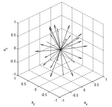
Fig. 13. Measured gravitational
acceleration vectors in ABF
The proposed algorithm is used
to evaluate the parameters of accelerometer parameters. The values of estimated
parameters are shown in Table 1.
Table. 1
Estimated
parameters by the proposed algorithm
|
αyz |
αzy |
αzx |
Sx |
Sy |
Sz |
bx [mg] |
by [mg] |
bz [mg] |
|
3.58×10⁻⁴ |
-7.29×10⁻³ |
4.62×10⁻⁴ |
1.0006 |
1.0030 |
0.9834 |
27.6253 |
-5.7079 |
-78.2870 |
In the datasheet of MPU 6050, the following values for the initial tolerance of
biases are given: bx=by=±50g and bz=±80g. As seen in Table 1, the obtained estimated values are
within these ranges. The differences between estimated biases on each axis are
significant.
The same set of data is used to obtain six
calibration parameters by the algorithm proposed in [8]. The estimated
parameters are shown in Table 2.
Table 2
Estimated parameters by the algorithm proposed in [8]
|
Sx |
Sy |
Sz |
bx [mg] |
by [mg] |
bz [mg] |
|
1.0008 |
1.0032 |
0.9835 |
28.1414 |
-5.4880 |
-77.2980 |
As could be seen from the above
tables, the estimated values of biases and scale factors by the two algorithms
are slightly different. To evaluate the accuracy of calibration, the following
calculations are made.
1. The calibrated measured
accelerations on each axis are calculated for all positions using the
parameters from the tables.
2. Double digital integration is
applied to calibrate accelerations in order to obtain the equivalent path on
each axis at each time moment [six(t), siy(t)
and siz(t)].
3. The errors in the overall
equivalent path for each position are calculated using the following formula ![]() .
.
4. Averaging over each position is
done at each time moment and the mean and standard deviation (ss) of errors in are obtained.
The calculated standard
deviation of errors of the overall equivalent path without calibration as a
function of time is shown in Fig. 14a. While the
calculated standard deviation of errors of the overall equivalent path with
calibration as a function of time is shown in Fig. 14b.
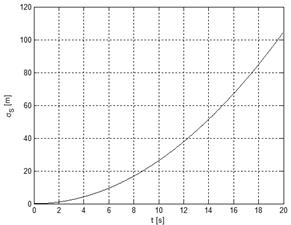
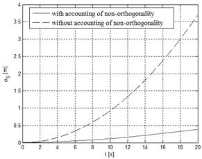
a) b)
Fig. 14. Standard deviation of errors of
the overall equivalent path.
The results show that the
standard deviation of errors of equivalent path without calibration at the end
of the period of 20 s is over 100 m. The standard deviation of errors in the
case of calibration with six parameters is less than 4 m and in the case of
calibration with nine parameters is less than 0.4 m. In this way, the accuracy
of path calculation, using the proposed algorithm of calibration, is more than
250 times better in comparison to the calculation without any calibration. The
improvement in accuracy of the proposed algorithm in comparison to the
algorithm with six parameters is about 10 times.
4. CONCLUSIONS
A procedure for MEMS
accelerometer static calibration, using a genetic algorithm, is proposed in
this paper. A fitness function for the genetic algorithm was defined. The
convergence of the estimates to the true values of parameters is very good.
Results from the simulations
and real accelerometer calibration showed that the proposed procedure provides
very good estimations of accelerometer parameters. The detailed studies showed
that two iterations are enough and that it is unnecessary to use more than 25
different positions of the accelerometer. Results of real accelerometer
calibration indicated much better accuracy when nine instead six parameters
were used.
References
1.
Bin Fang, Wusheng Chou, Li Ding. 2014. „An
Optimal Calibration Method for a MEMS Inertial Measurement Unit”. International Journal of Advanced Robotic
Systems 11(14): 1-14. DOI:
https://doi.org/10.5772/57516.
2.
Brunner
Thomas, Sebastien Changey, Jean-Philippe Lauffenburger, Michel Basset. 2015. “Multiple MEMS-IMU localization: Architecture comparison and performance
assessment”. In 22nd Saint
Petersburg International Conference on Integrated Navigation Systems, ICINS – Proceedings: 123-126.
State Research Center of the Russian Federation, Saint Petersburg, Russian
Federation. ISBN 9785919950233.
3.
Cai G., B.M. Chen, T.H. Lee. 2011. Unmanned
Rotorcraft Systems: Springer. ISBN 978-0-85729-634-4.
4.
Camps
F., S. Harasse. 2009. “Numerical calibration
for 3-axis accelerometers and magnetometers”.
In IEEE International Conference on
Electro/Information Technology. University of Windsor, Ontario, Canada. DOI: 10.1109/EIT.2009.5189614.
5.
Grankin Maxim, Elizaveta Khavkina,
Alexander Ometov. 2012. “Research of MEMS
Accelerometers Features in Mobile Phone”. In Proceeding of the 12th conference of FRUCT
association: 31-36. Finnish-Russian University Cooperation in
Telecommunication, Oulu, Finland. ISSN 2305-7254.ISBN 978-5-8088-0606-1.
6.
Prasant Kumar Mahapatra, Spardha, Inderdeep Kaur Aulakh, Amod Kumar, Swapna Devi. 2013. “Particle swarm optimization (PSO) based tool position error optimization”, International Journal of Computer
Applications 72(23): 25-32. ISSN 0975-8887.
7.
Marinov Marin, Zhivo Petrov. 2014. “An approach for static calibration of
accelerometer MMA8451Q”. In International conference AFASES:
189-192. “Henri Coanda” Air Force
Academy, Brasov, Romania. ISSN 2247-3173.
8.
Petrov
Zhivo, Liliana Miron. 2019.
“Opportunities of a genetic algorithm for static calibration of MEMS
accelerometers”. In International
annual scientific conference of Aviation Faculty: 346-353. Aviation
Faculty, National Military University, Dolna Mitroloia, Bulgaria, ISBN 978-954-713-123-1.
9.
Sinha Vikas, Maurya Avinash.
2017. “Calibration of Inertial Sensor by Using Particle Swarm Optimization
and Human Opinion Dynamics Algorithm”. In International Journal of Instrumentation and Control Systems 7(1):
1-13. DOI: 10.5121/ijics.2017.7101.
10. Tedaldi David, Alberto Pretto,
Emanuele Menegatti. 2014. “A robust and easy to
implement method for IMU calibration without external
equipments”. In Proceedings of IEEE
international conference on robotics and automation: 3042-3049. Hong
Kong, China. DOI: 10.1109/ICRA.2014.6907297. ISBN:
978-1-4799-3685-4. ISSN: 1050-4729.
11. Tian Jing, Wenshu
Yang, Zhenming Peng, Tao Tang, Zhijun
Li. 2016. “Application of MEMS Accelerometers and Gyroscopes in Fast
Steering Mirror Control Systems”. Sensors
16(4): 440. ISSN 1424-8220. DOI: https://doi.org/10.3390/s16040440.
12. Umeda Akira, Mike Onoe, Kohji
Sakata, Takehiro Fukushia, Kouichi Kanari, Hiroshi Iioka. Toshiyuki
Kobayashi. 2004. “Calibration of three-axis accelerometers using a
three-dimensional vibration generator and three laser interferometers”. Sensors and Actuators A: Physical
114(1): 93-101. ISSN: 0924-4247. DOI:
https://doi.org/10.1016/j.sna.2004.03.011.
13. Won Peter, Farid
Golnaraghi. 2010. “A triaxial
Accelerometer Calibration Method Using a Mathematical Model”. IEEE Transactions on Instrumentation and
Measurement 59(8): 2144-2153. ISSN: 0018-9456, ISSN: 1557-9662. DOI: 10.1109/TIM.2009.2031849.
14. Zhang Liguo, Wenchao Li, Huilian Liu. 2012.
“Accelerometer Static Calibration based on the PSO
algorithm”. In 2nd International
Conference “Electronic &
Mechanical Engineering and Information Technology”. Shenyang,
China. DOI:https://doi.org/10.2991/emeit.2012.119. ISBN
978-90-78677-60-4.
Received 04.09.2019; accepted in revised form 30.10.2019
![]()
Scientific
Journal of Silesian University of Technology. Series Transport is licensed
under a Creative Commons Attribution 4.0 International License