Article
citation information:
Sakno, O., Moysya, D.L.
Kolesnikova, T. Dynamic stability of a model of a tractor-lorry-trailer combination. Scientific Journal of Silesian University of
Technology. Series Transport. 2018, 99,
163-175. ISSN: 0209-3324. DOI: https://doi.org/10.20858/sjsutst.2018.99.15.
Olha SAKNO[1],
Dmitry L. MOYSYA[2], Tatiana KOLESNIKOVA[3]
DYNAMIC STABILITY
OF A MODEL OF A TRACTOR-LORRY-TRAILER COMBINATION
Summary. In this paper, we consider the mobility and
stability of a model of a tractor-lorry-trailer combination, consisting of a
two-axle tractor and a single-axle semi-trailer, and its possible stationary
states with fixed steering. A feature of this research is the study of a
non-linear mathematical model of a two-link tractor-lorry-trailer combination.
The set of steady-state conditions for the movement of the
tractor-lorry-trailer combination model is determined on the basis of the
developed mathematical model; it provides the necessary mobility for the
passage of the circular overall traffic lane. The range of stable steady-state
conditions of the road train is limited and the character of the loss of
stability in the direct motion of the road train (divergent, flutter) is
checked. The phase portraits of the system are constructed at different speeds,
which allow us to estimate the range of attraction for direct motion. Stability
issues are also considered, namely, the influence of the control parameters
(θ, v) on stability or instability.
Keywords: dynamic stability;
mobility of tractor-lorry-trailer combination; steady-state condition
1. INTRODUCTION
Fast and economical delivery of
indivisible wide loads in many industries is becoming increasingly important [1].
Road trains play a major role in solving this problem [2-5]. Their operation
can be complicated by design features, primarily the limited manoeuvrability of
long road trains in restricted urban conditions [6-8].
In this case, a double
(two-trailer) road train is considered, which consists of a leading link
(tractor) and a driven link (semitrailer).
The mathematical model of the
canonical road train is the object of research for many authors, where the
results of analysis of linearized models are mainly presented [9-13].
The specificity of this paper is
the study of the non-linear mathematical model of a double road train, whose
aim is to find possible rearrangements of the road train configuration in
different initial disturbances of phase variables. This requires non-standard
analysis methods (phase portrait construction and evaluation of the domain of
attraction for stable steady-state regimes).
The purpose of the paper is as
follows:
a) Investigate the manoeuvrability
and stability of the model of a double road train
b) Determine a set of
stationary traffic conditions, which provides the necessary manoeuvrability by
passing a circular overall lane
c) Estimate domains of attraction
for a stable steady-state regime
d) Check the type of stability loss
in direct motion (divergent, flutter)
2. CONSTRUCTION OF A
MATHEMATICAL MODEL FOR SEMI-TRAILER TRUCK MOTION
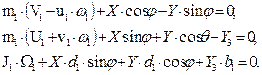
For the most complete description
of and research into possible stationary states of a semi-trailer truck (Fig.
1) with rigid steering, it is necessary to choose a suitable mathematical model
and applicable state variables (Fig. 2).
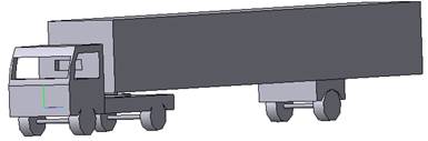
Fig. 1. Model of
semi-trailer truck
The front axle of the
tractor can be turned by an angle θ. The connection between the links is
carried out by a cylindrical hinge, which enables the free relative rotation of
the links in the plane of motion.
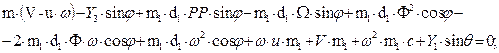
The configuration of
each link is described by coordinates xi and yi, its
centre-of-mass Сi and course angle ψi (it is
enclosed between the longitudinal axis of the corresponding link and the X-axis
of the fixed coordinate system).
The system parameters
are as follows:
v - longitudinal
velocity component of the centre of mass of the tractor
a; b - distance from the centre of mass of the tractor
to the attachment point of the front and back axles of the tractor
c - distance
from the centre of mass of the tractor to the hitch point with the back link
d1 - distance
from the centre of mass of the back link to the hitch point
2K - overall width of
the road train
kf - friction coefficient
k1, k2, k3 - the factors influencing
lateral skid on the axes
χ1,
χ2, χ3 - adhesion factors in determining the
force of lateral skid
θ - assignable wheels’ turning angle for the subordinate
module
Y1, Y2,
Y3 - lateral reaction of the highway area
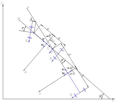
Fig. 2. Traffic plan of
a semi-trailer truck
If we assume that
С, С1 are the mass centres of the tractor and
semi-trailer), m, m1 are
the masses of the tractor and semi-trailer, I, I1 are the central
moments of inertia about the vertical axes, ω=ψ́, ω1=ψ́1 are
absolute angular velocities of the driving and driven links, and φ is the
angle of folding (it is enclosed between the longitudinal axes of the tractor
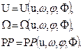
and semitrailer), then ![]() .
.
We set the absolute
velocities of points С, С1 by
their resolution along the axes of the corresponding bases:

 (1)
(1)
The differential
equation system of motion for the semi-trailer truck describes the variation in
phase variables (u, w ,φ, Φ),
where: u - cross speed of the centre of mass of the tractor (quasi-velocity); U
- its derivative in the moving coordinates; w - angular acceleration relative to the vertical axis; and Φ -
velocity of jack-knifing angle φ.
Among the different
theories for the rolling of elastically deformable wheels, the field of
axiomatics has become the most widespread, according to which the lateral
reaction Yi of the highway area is applied in tooth bearing centre
of the rolling elastic wheel, which is a function of slip angle δi.
The reduced angles of
lateral skid of the wheel axles are given by the following expressions:
![]() ;
;
![]() ; (2)
; (2)
 .
.
The dependencies of the
forces of lateral skid are of empirical origin [2] and can be approximated by
expressions (the strictly increasing function is the rate of the curve of
saturation):
![]() , (3)
, (3)
where Zi is the
reaction of the bearing area on the axes.
We neglect the
redistribution of normal reactions between the lateral wheels and instead
consider the lateral wheels of each axis that is replaced by one reduced wheel
with a centre in the middle of the axis:
Then:
![]() ;
;
![]() ; (4)
; (4)
![]() .
.
2.1. The derivation of
the system of equations in the normal Cauchy form
The derivation of the
differential equations for the plane-parallel motion of a semi-trailer truck is
performed by the cut set method [4].
Using this method, we
obtain the following equations for the plane-parallel motion, which in axial
projections are invariably associated with links for the tractor and
semi-trailer, respectively:
a) The motion equations
of the tractor are:
![]()
 (5)
(5)
b) The motion equations
of the trailer are:
 (6)
(6)
We eliminate the
internal forces X, Y of the interaction of subsystems from Eqs. (5) and (6), and we obtain a system of non-linear differential
equations in (7):
a) With variable
quantity v:
b) With variable
quantity u:
 (7)
(7)
c) With variable
quantity ω:

d) With a jack-knifing
angle:
Consider a uniform
motion, then v=const; therefore, V=0. We substitute into the system of
equations in (7) the value V=0 and solve it in relation to the higher
derivative (U, PP, Ω), where PP is the angular acceleration of the driven
link relative to the vertical axis.
We get a system of
equations in the normal Cauchy form (8):
 (8)
(8)
3. NUMERICAL ANALYSIS RESULTS OF
THE MATHEMATICAL MODEL OF THE ROAD TRAIN
Applying
the numerical methods of integration in the Maple package, we get the following
numerical analysis results for the mathematical model of a road train:
1. Locating a road train under circular
steady-state conditions of motion
Circular
trajectories of all points of a double road train on a road plane meet the
stationary solutions (that is, the equilibrium state, singular points and rest
points), in which ω=const, u=const, φ=const of the system with
v=const, and θ=const.
Setting
the system parameters:
m=6,500
kg; m2=36,500 kg; a=0.4 m; b=3.2 m; c=2.7 m; b1=2.8 m; d1=5.4
m;
v=4.5 m/s; θ=0.38; k1=160,000
H; k2=326,000 H; k3=365,000 H;
J=0.35∙m∙a∙b (kg∙m2);
J2=0.8∙m1∙d1∙b1
(kg∙m2); ci=0.8; К=1.5 m
The given
parameters and values of the control parameters v and θ are substituted in
the systems of equations in (8), which we then solve to obtain the following
results.
Thus, the circular
steady-state conditions correspond to the values of v=4.8 m/s and θ=0.42
rad; the trajectory of the tractor’s centre-of-gravity motion in the
plane of the road and the position of the tractor are shown in Fig. 3.
We obtain a circular
stationary regime with v=5 m/s and θ=0.36 rad, as shown in Fig. 4.
The attitude of the road
train is shown when moving along a circular corridor in Figs. 3 and 4, limiting
the dimensions of which correspond to EU standards. It can be seen that, for
the given control parameters, in the first case, the semi-trailer and, in the
second case, the tractor and semi-trailer go beyond the dimensions of the
corridor.
|
|
|
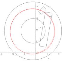
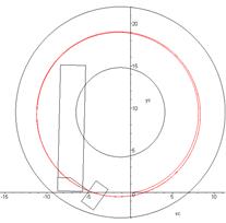
Fig. 3. Trajectory of
the tractor’s centre-of-gravity motion in the plane of the road
(v=4.8 m/s and
θ=0.42 rad)
|
|
|
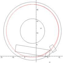
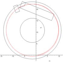
Fig. 4. Trajectory of
the tractor’s centre-of-gravity motion in the plane of the road
(v=5 m/s and
θ=0.36 rad)
Thus,
there are values of v and θ at which the road train will pass a circular
corridor, fitting its dimensions.
Control
parameters were selected by the method of progressive approximation v=5 m/s and
θ=0.36 rad, which corresponds to a circular steady-state condition with a
trajectory. This is shown in Fig. 5.
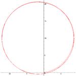
Fig. 5. Trajectory of
the tractor’s centre-of-gravity motion in the plane of the road
(obtained
by numerical integration in the Maple package)
This trajectory
corresponds to the passage by a road train of a circular corridor, the
dimensions of which correspond to EU standards, as shown in Fig. 6.
|
|
|
|
а) |
b) |
|
|
|
|
c) |
d) |
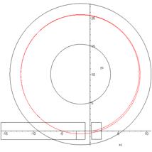
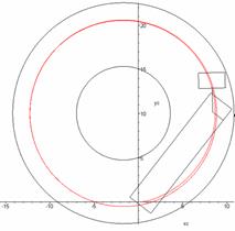
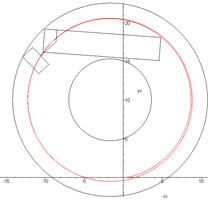
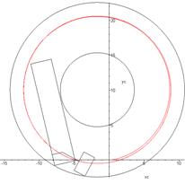
Fig.
6. A double
road train passes a circular corridor
(corridor dimensions comply with EU standards): a) entering the corridor; b-d)
passing of the corridor
2. Determination of
the stability range of the rectilinear regime in the parameter space
(analytical and numerical definition of the critical speed of rectilinear
motion)
The linear approximation of the initial system is used for the numerical
determination of critical velocity. The eigenvalue spectrum is determined for
the different parameter value v. This
approach makes it possible to establish the existence of stability
(instability) for a pattern of design factor. The method of interval bisection
facilitates the determination of the moment of the loss of stability (vkr)
[3].
Take, for example, the following set of parameters: m=6,500
kg; m2=36,500 kg; a=0.4 m; b=3.2 m; c=2.7 m; b1=2.8 m; d1=5.4
m; k1=160,000 H; k2=226,000 H; k3=270,000
H; J=0.35∙m∙a∙b (kg∙m2);
J2=0.8∙m1∙d1∙b1
(kg∙m2); ci=0.8;
θ=0; К=1.5 m
This corresponds to the eigenvalue spectrum at the value v=20 m/s:
![]()
The eigenvalue spectrum of the system (8) at v=20 m/s is shown in Fig. 7.
Since the roots of the performance
equation of a system experiencing variations are negative real parts, according
to the Lyapunov theorem, the linear traffic condition is stable.
Fig. 7. The eigenvalue spectrum of
the system (8) at v=20 m/s.
We have at v=35 m/s:
![]()
If one real root is positive, then the regime is unstable.
The eigenvalue spectrum of the system (8) at v=35 m/s is shown in Fig.
8.
Consequently, there is a loss of stability in the linear motion in the
speed range 20 m/s<v<35 m/s. The zero eigenvalue corresponds to the
velocity value vкр (the so-called critical case of one
zero root involves a divergent loss of stability). In this case, the initial
perturbations of the phase variables are grown aperiodically. The case of a
couple of complex eigenvalues with zero real parts corresponds to a periodic
increase in the initial perturbations of the phase variables, leading to flutter instability.
We have at v=31 m/s:
![]()
Fig. 8. The eigenvalue spectrum of the system (8) at v=35 m/s
The eigenvalue spectrum of the system (8) at v=31 m/s is shown in Fig.
9.
One of
the real roots with some degree of accuracy is equal to zero, that is, a
divergent loss of stability is going to occur at the velocity value vkr=31
m/s.
The
analytic expression for determining the critical velocity is given by:
 . (9)
. (9)
Fig. 9. The eigenvalue spectrum of the system (8) at v=31 m/s
The
numerical value of the critical velocity for the selected parameters of the
system is vkr=30.97 m/s. This result confirms the results of the
trial-and-error method.
It
follows from (9) that vkr depends on a certain design factor. We
analyse how the value vkr changes with the variation in the
parameters L1 and m1.
If we
only change the mass of the semi-trailer in the design factors of the system,
as presented in Fig. 10, we obtain the dependence of critical velocity on the
mass of the semitrailer vkr=f(m1).
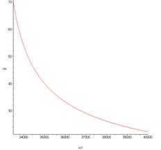
Fig. 10. Graph of the dependence of critical
velocity
on
the mass of the semitrailer vkr=f(m1)
If we
assume m1=33,000 kg, we can determine that the divergent loss of
stability comes at a value of vkr=123 m/s. The flutter loss of
stability under certain conditions could happen earlier than at the divergent
stage. As such, it is necessary to check what happens with a flutter loss of
stability at lower values vkr, as well as determine the eigenvalue
spectrum of the system under vkr=120 m/s:
![]()
Since
the real parts of the roots are negative, the flutter loss of stability does
not set in, that is, the regime is stable.
Changing
the position of the centre of gravity of the semi-trailer, that is, varying the
ratio d1/b1, we get the following dependence of the
critical velocity:
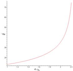
Fig. 11. Graph of the dependence of the critical
velocity on the ratio d1/b1 (vkr=f (d1/b1))
From
the graph, it follows that critical speed value will decrease when the
semi-trailer’s centre of gravity in relation to the hitch point is
approximated.
4. MODELLING OF PHASE PORTRAITS OF
THE MODEL (ANALYSIS OF THE STABILITY REGION OF THE RECTILINEAR REGIME)
The system (7) is
allowed an obvious solution {v=const; u=0; w=0; q=0; φ=0; Φ=0}
with balanced longitudinal forces (X1=0; X2=0; X3=0). This corresponds to the uniform rectilinear
motion of the road train (stationary rectilinear mode). The set of
steady-state conditions is determined by the system (7) in which we substitute
the following values: U=0; w=0; Φ=0; PP=0.
We take the control
parameter of the system v=20 m/s and θ=0 and construct a phase portrait in
the space of variables (u, ω). The system comprises three steady-state
conditions. These regimes correspond to three singular points on the phase
plane: at the origin of coordinates of the stable node (it corresponds to a
rectilinear regime) and two saddle points that are symmetrically located (they
correspond to unstable circular regimes). Saddle special points are approximated
to the origin of coordinates according to an increase in the parameter v. The stability of the rectilinear
regime is wrecked at v=vkr. The domain of stability of the
rectilinear regime limits the incoming separatrix of the saddle points [6], as
shown in Fig. 12.
The
coordinates of the saddle points were numerically determined using the Maple
package as a solution to the system of non-linear equations (7):
(u=-5.279; φ=-0.0653;
ω=0.2198); (u=5.279; φ=0.0653; ω=-0.2198)
The phase portrait of
the system at v>vkr is
discussed in Fig. 13.
The system is one
unstable rectilinear traffic condition, which corresponds to a saddle singular
point at the origin of coordinates. The initial perturbations grow
aperiodically, which should correspond to the phenomenon of skidding. The phase
variables in this case are close to the stable separatrices of the saddle. The
coordinates of the saddle singular point are as follows: (u=0; φ=0;
ω=0).
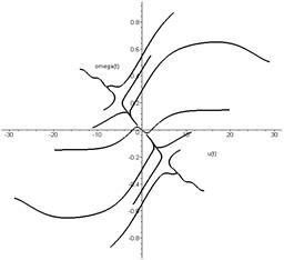
Fig. 12. Phase portrait of the system at subcritical velocity
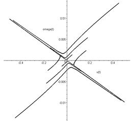
Fig. 13. Phase portrait of the system at supercritical speed
5. CONCLUSION
Stability problems,
namely, the influence of motion parameters on stability (instability), are
considered. The graphs of the dependence of the critical velocity on the mass
of the semi-trailer and its geometric parameters are constructed. These
dependencies make it possible to determine the design factors of the system.
This corresponds to a divergent loss of stability. Flutter loss of stability
under the considered parameters is not found.
Phase portraits of the
system are constructed at different speeds, which makes it possible to estimate
the domain of attraction of linear motion. The domain of attraction of the
rectilinear regime is limited by separatrices. The initial values of the phase
variables can be estimated in phase portraits, leading to the conclusion that
the system exists in the stability domain. The implementation of these initial
disturbances can result from external influences (crosswind, impact with the
edge of the roadway etc.).
The
values of the speed (v) and the steering angle (θ) are determined for the
selected design factors of the model, which ensures the passage of the road
train along the circular overall corridor.
References
1.
Havenga
J.H. 2018. “Logistics and the future: The rise of macrologistics”. Journal of
Transport and Supply Chain Management
12(a336).
2.
Day
A. 2014. “Braking system design for vehicle and trailer
combinations”. In: Braking of Road Vehicles. Edited by A. Day 67-96. Oxford: Elsevier. ISBN: 978-0-12-397314-6. DOI: https://doi.org/10.1016/B978-0-12-397314-6.00004-8.
3.
Эллис
Д. 1975. Управляемость
автомобиля.
Москва:
Машиностроение.
[In Russian: Ellis D. 1975. Vehicle Handling. Moscow:
Mashinostroenie.]
4.
Hu
Xing-jun, Peng Qin, Lei Liao, Peng Guo, Jing-yu Wang, Bo Yang. 2014.
“Numerical simulation of the aerodynamic characteristics of heavy-duty
trucks through viaduct in crosswind”. Journal of
Hydrodynamics Series B 26(3): 394-399. ISSN: 1001-6058. DOI: https://doi.org/10.1016/S1001-6058(14)60044-5.
5.
Mathisen
T.A., T.E. Sandberg Hanssen, F. Jørgensen, B. Larsen. 2015.
“Ranking of transport modes ‐ Intersections between price curves for transport by
truck, rail, and water”. Transport\Transporti
Europei 57(1).
6.
Лобас
Л., В.
Вербицкий 1990. Качественные
и
аналитические
методы в динамике
колесных
машин. Киев.
Наукова
думка. [In Russian: Lobas L., V. Verbitskiy.
1990. Qualitative and Analytical Methods
in the Dynamics of Wheeled Vehicles. Kiev: Naukova Dumka.]
7.
Рокар
И. 1990. Неустойчивость
в механике.
Москва:
Иностранная
литература.
[In Russian: Rokar I. 1990. Instability
in Mechanics. Moscow: Inostrannaya Literature.]
8.
Rackham D.H.,
D.P. Blight. 1985. “Four-wheel drive tractors”. Journal of
Agricultural Engineering Research 31(3): 185-201. ISSN: 0021-8634. DOI: https://doi.org/10.1016/0021-8634(85)90087-3.
9.
Ritzen
Paul, Erik Roebroek, Nathan van de Wouw, Zhong-Ping Jiang, Henk Nijmeijer.
2016. “Trailer steering control of a tractor-trailer robot”. IEEE
Transactions on Control Systems Technology 24(4):
1240-1252. ISSN: 1063-6536. DOI: 10.1109/TCST.2015.2499699.
10. Вербицкий
В. Г., Л. Г.
Лобас. 1987.
“Бифуркации
и
устойчивость
стационарных
состояний
связки
катящихся упруго-деформированных
тел”. Прикладная
механика 8: 101-106. ISSN:
0032-8243. [In Russian: Verbitskiy V., L. Lobas
1987. “Bifurcations and stability of stationary states of a bundle of
rolling elastically deformed bodies”. Prikladnaya
mekhanika 8: 101-106. ISSN: 0032-8243.]
11. Вербицкий
В., Л.
Лобас. 1996.
“Вещественные
бифуркации
двухзвенных
систем с
качением”. Прикладная
математика и
механика 3: 418-425. ISSN:
0032-8235. [In Russian: Verbitskiy V., L.
Lobas 1996. “Real bifurcations of two-link systems with rolling”. Prikladnaya matematika i mekhanika 3:
418-425. ISSN: 0032-823.]
12. Вербицкий
В., М.
Загороднов 2007.
“Определение
и анализ устойчивости
круговых стационарных
режимов
движения
модели седельного
автопоезда”. Вестник
Донецкого
института
автомобильного
транспорта 1:
10-19. ISSN: 2219-8180. [In Russian:
Verbitskiy V., M. Zagorodnov. 2007.
“Determination and analysis of the stability of circular stationary modes
of motion of the model of a semitrailer road train”. Vestnik Donetskogo instituta avtomobilnogo transporta 1: 10-19.
ISSN: 2219-818.]
13. Wu Tong, John Y. Hung. 2017. “Path
following for a tractor-trailer system using model predictive control”.
In: IEEE SoutheastCon 2017. 30 March to 2 April 2017. Charlotte, NC,
USA. ISSN: 1558-058X. DOI: 10.1109/SECON.2017.7925337.
Received 17.02.2018; accepted in revised form 15.05.2018
![]()
Scientific
Journal of Silesian University of Technology. Series Transport is licensed
under a Creative Commons Attribution 4.0 International License