Article citation information:
�ochowska, R., Socz�wka, P. Analysis of selected transportation network structures based on graph measures. Scientific Journal of Silesian University of Technology. Series Transport. 2018, 98, 223-233. ISSN: 0209-3324. DOI: https://doi.org/10.20858/sjsutst.2018.98.21.
Renata �OCHOWSKA[1],
Piotr SOCZ�WKA[2]
ANALYSIS
OF SELECTED TRANSPORTATION NETWORK STRUCTURES BASED ON GRAPH MEASURES
Summary. The structure of transportation networks has been the subject of analysis for many years, due to the important role that it plays in assessing the efficiency of transportation systems. One of the most common approaches to representing this structure is to use graph theory, in which elements of transportation infrastructure are depicted by a set of vertices and edges. An approach based on graph theory allows us to assess the structure of a transportation network in terms of connectivity, accessibility, density or complexity. In the paper, different transportation network structures are assessed and compared, based on graph measures.
Keywords: transportation network, graph theory, graph and topology measures
1. INTRODUCTION
A transportation network is usually understood
as a set of transportation points, with connections between them, in the form
of paths or routes, designed for travel by people, cargo shipments and the
passage of vehicles [20]. The spatial structure of such a network corresponds
to the connections that exist between the elements of transportation
infrastructure in the geographical space. This means that elements of the
transportation network are also elements of land use in the area in which they
are located [5]. The volume of traffic flows, expressed by the number of
travelling people, as well as moving vehicles, or by the mass of carried goods
in a given unit of time, is one of the measures of transportation network
performance.
The efficiency of the entire transportation
system in the area under analysis is largely determined by the structure of its
transportation network. The denser and more consistent the network, the greater
the number of connections between two selected vertices. This has a significant
impact on the possibility of reducing traffic congestion by moving traffic onto
alternative roads, which in turn means shorter travel time. This explains why
the analysis of transportation network structures has been the subject of
intensive research for many decades [1,6-9,22,24].
The article analyses the assessment of selected
structures of a transportation network based on graph measures. The network
models correspond to real transportation systems. The analysis is carried out
in terms of the possibility of using different types of graph measures when
assessing the propagation of disturbances in the transportation network.
2. REPRESENTATION OF THE TRANSPORTATION NETWORK
STRUCTURE�
The physical topology of a network, which is
understood as the arrangement of nodes and links in the network, is based on
point and linear transportation infrastructure objects. The aim of the study is
to define the scope of the representation of the infrastructure�s elements and
the connections between them. Therefore, the structure of the network may be
both very simplified and particularly complex. Thus, depending on the adopted
criteria for the classification of transportation systems, scales and
aggregation level, a transportation node may be a single intersection, a bus
stop, a railway station, a road junction, an airport, a logistics centre or
even a whole city. In turn, the link may be a single traffic lane, a railway
track, a communication route or a corridor connecting important transportation
nodes. When designing a network model, the proper representation of location,
direction and connections is of particular importance. It is also worth noting
that the topology of a network model should be as close as possible to the
structure of the real network it represents [18].
The structure of the transportation network can
be mapped by using various mathematical tools. One of the most commonly and
intuitive approaches is to represent the transportation system of the studied
area using graph theory [12,25]. Graph methods has been used to map and study
the spatial structure of transportation networks since the 1960s [10,13]. In
Poland, they have been used, for example, to assess the topological
accessibility of the railway network of the West Pomeranian Voivodeship [19], former
Pozna� Province [15,16] and Silesia [21].
The main requirement of topological analysis is
to represent an existing transportation network as an abstract set of points
(nodes or vertices), connected by a set of lines (segments, edges or arcs). In
the graph theory approach, attention is primarily centred on the arrangement of
connections between nodes, which allows for the use of undirected graphs.
Metric and capacity characteristics are also often ignored [2].
Two basic approaches to the representation of a
transportation network structure using graph theory are found in the literature
[23]:
-
Primal, in which the nodes of the network are
represented in the form of vertices, and links in the form of arcs or edges
-
Dual, in which the sections of the network are
represented in the form of vertices, and nodes in the form of arcs or edges
For the purpose of analysing the values of
selected graph measures for various structures of a transportation network, a
set of numbers relating to the types of structures has been determined as
follows:
![]() ��������������������������������������������������������� (1)
��������������������������������������������������������� (1)
where![]() �is the number for structure type, and
�is the number for structure type, and![]() �is the number for all structure types under
analysis. Therefore, using the primal approach to mapping the structure of the
transportation network, the
�is the number for all structure types under
analysis. Therefore, using the primal approach to mapping the structure of the
transportation network, the ![]() -th structure of the network may be
described in the form of a graph:
-th structure of the network may be
described in the form of a graph:
![]() ��������������������������������������������� (2)
��������������������������������������������� (2)
where![]() �is the set of vertices of graph
�is the set of vertices of graph ![]() ,
,![]() is the set of edges of graph
is the set of edges of graph ![]() . Both the vertices and the edges
are sequentially numbered. Therefore, the set
. Both the vertices and the edges
are sequentially numbered. Therefore, the set ![]() �contains subsequent numbers for the vertices
of graph
�contains subsequent numbers for the vertices
of graph ![]() , i.e.:
, i.e.:
![]() �������������������������������������������� (3)
�������������������������������������������� (3)
where
![]() �is the number of a vertex of graph
�is the number of a vertex of graph ![]() ,
,![]() �is the number of the last vertex (in the set
of vertex numbers in ascending order) corresponding to the size of the set
�is the number of the last vertex (in the set
of vertex numbers in ascending order) corresponding to the size of the set ![]() , and the set
, and the set ![]() �contains subsequent numbers for the edges of
graph
�contains subsequent numbers for the edges of
graph ![]() , i.e.:
, i.e.:
![]() ��������� ���������������������������������� (4)
��������� ���������������������������������� (4)
where![]() �is the number for an edge of graph
�is the number for an edge of graph ![]() , and
, and![]() �is the number for the last edge (in the set of
edges numbers in ascending order) corresponding to the size of the set
�is the number for the last edge (in the set of
edges numbers in ascending order) corresponding to the size of the set ![]() .
.
The mathematical model of the transportation
network should be constructed in such a way as to enable the identification of
its elements, the description of its spatial structure and the assignment of
specific characteristics to its individual elements [26].
3. MEASURES OF A TRANSPORTATION NETWORK
STRUCTURE�
There
are many measures that can be used to assess the structure of the
transportation network and analyse its efficiency. Some of them take into
account spatial features (distance, surface), as well as the level of activity
(traffic), while others solely rest on the topological dimension of the
network. They may be applied to [18]:
-
The expression of the relationship between values and
the network structures they represent
-
The comparison of different transportation networks at
a specific point in time
-
The comparison of the evolution of a transportation
network at different points in time
The representation of the structure
of the transportation network in the form of graph enables a set of functions
to be assigned, which correspond to the properties (characteristics) of the
elements of this structure in relation to each vertex and/or edge of the graph.
These characteristics are also used to assess the structure of the
transportation network. In order to conduct comparative analyses of the
topology of entire networks or their parts, the measures at the network level
are particularly important. Among the groups of indices for assessing the
structure of a transportation network are graph measures, which are
particularly important because of the representation of the network in the form
of a graph.
One of the most important
characteristics of a transportation network is its level of connectivity, which may be described as the degree of
connections in a particular area or a measure of how many components of the
transportation network are connected to each other [3,17]. The more connected
networks there are, the shorter the travel times and costs. Moreover,
connectivity plays an important role in the social and economic development of
regions [17]. Three measures, based on graph theory, were initially developed
by Kansky [10,11] and can be used to assess the connectivity of a
transportation network [4,11,18]: alpha, beta and gamma measures. It is worth
noting that all of them are ratios, that is, they represent a relation between
distinguishable elements of a network [11,18].�
The alpha measure ![]() �compares the number of cycles in the network
represented by the graph
�compares the number of cycles in the network
represented by the graph ![]() �with maximum number of cycles [11,18]. This
measure can range from 0 to 1. Values close to 1 indicate a well-connected
network; however,
�with maximum number of cycles [11,18]. This
measure can range from 0 to 1. Values close to 1 indicate a well-connected
network; however, ![]() �does not usually equal 1. For simple and less
connected networks (for example, tree networks), values of
�does not usually equal 1. For simple and less
connected networks (for example, tree networks), values of ![]() �are close to 0.
�are close to 0.
The alpha measure may be calculated
based on the following formula:
![]() ������������������������� (5)
������������������������� (5)
where![]() �is the number of edges in a graph
�is the number of edges in a graph ![]() , wherein
, wherein ![]() ;
;![]() �is the number of vertices in a graph
�is the number of vertices in a graph ![]() , wherein
, wherein ![]() ; and
; and ![]() �is the number of isolated subgraphs in a graph
�is the number of isolated subgraphs in a graph
![]() . The alpha measure is often
expressed as a percentage value, which denotes the percentage of maximum
connectivity.
. The alpha measure is often
expressed as a percentage value, which denotes the percentage of maximum
connectivity.
The second graph measure, the beta measure ![]() , expresses the relation between a
certain number of edges and the number of vertices in a graph
, expresses the relation between a
certain number of edges and the number of vertices in a graph ![]() �[4,18]. It is one of the simplest measures
used to evaluate the connectivity of transportation networks [11]. It may be
calculated based on the following formula:
�[4,18]. It is one of the simplest measures
used to evaluate the connectivity of transportation networks [11]. It may be
calculated based on the following formula:
�
![]() ������������������������������� (6)
������������������������������� (6)
where ![]() �is the number of edges in a graph
�is the number of edges in a graph ![]() , wherein
, wherein ![]() ; and
; and![]() �is the number of vertices in a graph
�is the number of vertices in a graph ![]() , wherein
, wherein ![]() .
.
Similar to
the alpha measure, higher values of the beta index characterize well-connected
networks [4,11]. For planar graphs, the maximum value of the beta index is 3,
whereas, for non-planar graphs, its values are infinite. All disconnected
graphs have values of the beta measure smaller than 1, while a perfect grid
network may have values of the beta measure around 2.5. For network planning
purposes, values of about 1.4 for the beta measure are acceptable [3].
The third graph measure developed by
Kansky, the gamma measure ![]() , expresses the relation between an
observed number of edges in the network and the maximum possible number of
edges [12,19]. Similar to the alpha measure, it ranges from 0 to 1, with 1
denoting a completely connected network and 0 denoting a poor level of connectivity
[11]. It is determined as follows:
, expresses the relation between an
observed number of edges in the network and the maximum possible number of
edges [12,19]. Similar to the alpha measure, it ranges from 0 to 1, with 1
denoting a completely connected network and 0 denoting a poor level of connectivity
[11]. It is determined as follows:
�
![]() ����������������������� (7)
����������������������� (7)
where ![]() �is the number of edges in a graph
�is the number of edges in a graph ![]() , wherein
, wherein ![]() ; and
; and![]() �is the number of vertices in a graph
�is the number of vertices in a graph ![]() , wherein
, wherein ![]() . It is worth noticing that Formula
(7) is applicable to planar graphs [11]. Usually, the gamma measure is
expressed as percentage values.
. It is worth noticing that Formula
(7) is applicable to planar graphs [11]. Usually, the gamma measure is
expressed as percentage values.
Different graph-based measures take
into consideration the network as a whole. Example of such measures may be the eta measure ![]() , which is an average length of a
link in a transportation network [4,11]. It may be calculated based on the
following formula:
, which is an average length of a
link in a transportation network [4,11]. It may be calculated based on the
following formula:
�
![]() ����������������������������� (8)
����������������������������� (8)
where![]() �is the total length of the graph
�is the total length of the graph ![]() , i.e., the sum of the length of all
edges from the set
, i.e., the sum of the length of all
edges from the set ![]() ; and
; and ![]() �is the number of edges in a graph
�is the number of edges in a graph ![]() , wherein
, wherein ![]() . The total length
. The total length ![]() �of the graph
�of the graph ![]() �is a very important characteristic of the
transportation network structure from the point of view of its efficiency.
According to [4], the longer the edges in the network, the better it is to
ensure the maximum speed of a given link. The total length
�is a very important characteristic of the
transportation network structure from the point of view of its efficiency.
According to [4], the longer the edges in the network, the better it is to
ensure the maximum speed of a given link. The total length ![]() �is also taken into account in the calculation
of the pi measure
�is also taken into account in the calculation
of the pi measure ![]() , which expresses the relationship
between the total mileage of a transportation network and its diameter [11,18].
It may be determined based on the following formula:
, which expresses the relationship
between the total mileage of a transportation network and its diameter [11,18].
It may be determined based on the following formula:
![]() ������������������������������� (9)
������������������������������� (9)
where ![]() �is the total length of the graph
�is the total length of the graph ![]() , and
, and![]() �is the length of a diameter of a graph
�is the length of a diameter of a graph ![]() , i.e., the length of the shortest
path between the two most distanced vertices from the set
, i.e., the length of the shortest
path between the two most distanced vertices from the set ![]() .
.
The pi measure equals 1 for less
complicated networks. Greater values are ascribed to more complex
transportation networks [11].
Another important measure based on
graph theory is the graph density ![]() , which is understood as the ratio
of the number of its edges to the largest possible number of edges that may be
stretched on the vertices of the graph
, which is understood as the ratio
of the number of its edges to the largest possible number of edges that may be
stretched on the vertices of the graph ![]() �[26]. Therefore, this measure is calculated
based on the following formula:
�[26]. Therefore, this measure is calculated
based on the following formula:
![]() ����������������� (10)
����������������� (10)
where![]() �is the number of edges in a graph
�is the number of edges in a graph ![]() , wherein
, wherein ![]() ; and
; and![]() �is the number of vertices in a graph
�is the number of vertices in a graph ![]() , wherein
, wherein ![]() .
.
The density of the graph may also be determined
in relation to the real area ![]() �occupied by the transportation network, as
represented by the graph
�occupied by the transportation network, as
represented by the graph ![]() . Hence, nodal and edge graph
density can be distinguished. The vertices and edges of the graph
. Hence, nodal and edge graph
density can be distinguished. The vertices and edges of the graph ![]() �may represent point and linear elements of the
transportation infrastructure belonging to different transportation subsystems.
�may represent point and linear elements of the
transportation infrastructure belonging to different transportation subsystems.
Nodal graph density ![]() �is the relation between a number of vertices
and the area of the network. It may be calculated based on the following
formula:
�is the relation between a number of vertices
and the area of the network. It may be calculated based on the following
formula:
![]() ���������������������������������� (11)
���������������������������������� (11)
where![]() �is the number of vertices in a graph
�is the number of vertices in a graph ![]() , wherein
, wherein ![]() ; and
; and![]() �is the size of the area occupied by the
transportation network, as represented by the graph
�is the size of the area occupied by the
transportation network, as represented by the graph ![]() .
.
Edge graph density ![]() �is the relation between a number of edges and
the area of the network. It may be calculated based on the following formula:
�is the relation between a number of edges and
the area of the network. It may be calculated based on the following formula:
![]() ���������������������������������� (12)
���������������������������������� (12)
where![]() is the number of edges in a graph
is the number of edges in a graph ![]() , wherein
, wherein ![]() ; and
; and![]() �is the size of the area occupied by the
transportation network represented by the graph
�is the size of the area occupied by the
transportation network represented by the graph ![]() .
.
Network density ![]() �is yet another measure, which is understood as
the relation between the total length of the graph
�is yet another measure, which is understood as
the relation between the total length of the graph ![]() �and the area of the network. It may be
calculated based on the following formula:
�and the area of the network. It may be
calculated based on the following formula:
![]() ������������������� (13)
������������������� (13)
where![]() �is the total length of the graph
�is the total length of the graph ![]() , and
, and ![]() �is the size of the area occupied by the
transportation network, as represented by the graph
�is the size of the area occupied by the
transportation network, as represented by the graph ![]() .
.
Network density is a measure of the
development of a transportation network. Highly developed networks have higher
values of ![]() �[11]. Density may be also important in
determining the accessibility of a transportation system [14].
�[11]. Density may be also important in
determining the accessibility of a transportation system [14].
4. CASE STUDY
Four
different transportation network structures (mesh, tree, hub and spoke, and
linear) have been chosen in order to conduct a comparative analysis. The
network models have been developed on the basis of real communication systems
and chosen on the basis that the size of their respective area was similar. This
has allowed us to compare the values of network density and graph-based
measures. The analysed structures are presented in Figure 1.
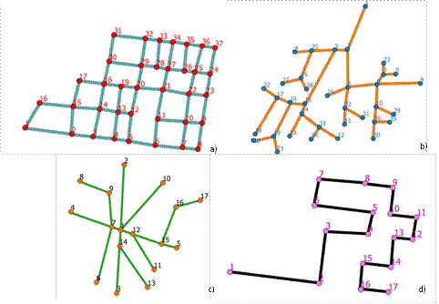
Fig. 1. Different types of
transportation network structure chosen for analysis:
a) mesh, b) tree, c) hub and spoke,
d) linear
Source: Own research
The selected characteristics for
each transportation network structure, as presented in Figure 1), are set
out in Table 1. They have been used to calculate the measures according to
Formulas (5)-(13).
Tab. 1
Values of selected
characteristics for the analysed types of transportation
network structure
|
Characteristics |
Type of transportation network structure� |
|||
|
Mesh
|
Tree
|
Hub and spoke
|
Linear
|
|
|
Number
of vertices
|
37 |
36 |
17 |
17 |
|
Number
of edges
|
58 |
35 |
16 |
16 |
|
Length
of graph
|
5.990 |
5.079 |
3.091 |
2.456 |
|
Size of
the area
|
0.264 |
0.293 |
0.252 |
0.270 |
|
Diameter
|
1.181 |
1.047 |
0.884 |
2.456 |
The
results of the analysis are presented in Table 2. The measures allow us to
assess the transportation network structures from different aspects, i.e.,
connectivity of the network, and its complexity or accessibility.
Tab. 2
Values of the selected graph
measures for different structures of transportation networks
|
Graph measure |
Type of transportation network structure |
|||
|
Mesh
|
Tree
|
Hub and spoke
|
Linear
|
|
|
Alpha
measure
|
0.32 |
0.00 |
0.00 |
0.00 |
|
Beta measure
|
1.57 |
0.97 |
0.94 |
0.94 |
|
Gamma measure
|
0.55 |
0.34 |
0.36 |
0.36 |
|
Eta measure
|
0.10 |
0.15 |
0.19 |
0.15 |
|
Pi measure
|
5.07 |
4.85 |
3.50 |
1.00 |
|
Graph density
|
0.09 |
0.06 |
0.12 |
0.15 |
|
Nodal graph density
|
140.15 |
122.87 |
67.46 |
62,69 |
|
Edge graph density
|
219.70 |
119.45 |
63.49 |
59,26 |
|
Network density
|
22.69 |
17.33 |
12.27 |
9.10 |
According to the calculated values of the
alpha, beta and gamma measures, the network with the highest level of
connectivity is the mesh network. Only in instances involving such a structure
does the beta measure exceed 1.00 and alpha measure exceed 0.00. The value of
the beta measure for the mesh network (1.57) is characteristic for connected
graphs and relatively close to 1.40, which is a good value for planning
purposes. However, it is still significantly smaller that the value for a
perfect grid. In terms of the other structures, the beta measures for the tree
network, hub and spoke network, and linear network are smaller than 1.00 and
similar to each other. Moreover, for these network structures, the alpha
measure equals 0.00, which is normal for tree networks and other less connected
networks (such as linear networks) [11]. Furthermore, the value of the gamma
index for the mesh network is significantly higher than for other networks.
There is no significant difference in the values of the gamma measure for the
tree network, hub and spoke network and linear network.
On the other hand, the value of the eta measure
for the mesh network is the smallest. This denotes that, in such a
transportation network structure, the average length of a link is shorter than
for other structures. However, it is worth noting that the mesh network has a
significantly larger number of edges and vertices in comparison to other
structures with a relatively similar size of area. Although edges are shorter,
they are much better connected to each other.
The mesh network has the densest structure,
which relates to the fact that, in a given area of a transportation network, there
are many short edges. The second densest network is the tree network; however,
there is no significant difference between the tree network and the hub and
spoke network. The least dense structure is the linear network.
The most complex network, based on the pi
measure, is the mesh network. The second most complex network is the tree
network, with a relatively similar pi measure result to the mesh network. The
hub and spoke network is the least complex. For the linear network, the pi
measure equals 1.00, which is normal for this type of structure as the diameter
equals the length of the graph [11].
Mesh and tree networks have a significantly
higher number of vertices per square kilometre. Less complex networks, i.e.,
the hub and spoke network and the linear network, tend to have a smaller number
of vertices in a similar area.
The mesh network is characterized by the
highest level of connectivity. Such a transportation network structure ensures
that the access to all vertices is quite easy; however, it also covers the
biggest part of a given area with edges (roads, railway etc.). Tree or hub and
spoke networks are not connected at a satisfactory level. This means that users
of such transportation networks have to travel longer, which also means higher
costs of transportation. Furthermore, in the case of linear networks,
connectivity is not satisfactory and accessibility to vertices is limited.
5. CONCLUSIONS
Analysing the structure of transportation
networks is an important subject of research. Typically, transportation
networks are represented, using graph theory, as a set of vertices and edges or
arcs, which represent real objects in the transportation infrastructure, such
as roads, intersections and bus stops. Therefore, measures based on graph theory
allow us to assess and compare different structures of a transportation
network.
Four different structures, which are common in
transportation systems all over the world, have been analysed and evaluated.
Nine graph-based measures have been used in order to reveal characteristic
features of the analysed structures. The study showed significant differences
in the level of connectivity or complexity among these structures.
The measures may be also used to assess
accessibility within a given transportation network. This in turn may have an
influence on the time or cost of transportation. As each transportation network
structure has certain unique features, it is important to perform an analysis
of these structures in order to reveal these features and make the best use of
them. This may influence the whole transportation system, of which a
transportation network is an important part.
The issues presented in the article require
further research. Of particular importance are aspects related to the method of
dividing the transportation network into smaller parts, taking into account the
network hierarchy. There is also a need to develop a comprehensive method of
assessing the structure of a transportation network, in which other factors
(e.g., traffic volume, area scale, level of aggregation) are taken into
account.
References
1.
Boora A., I.
Ghosh, S. Chandra. 2017. �Clustering Technique: An Analytical Tool in Traffic
Engineering to Evaluate the Performance of Two-Lane Highways European� Transport\Transporti
Europei 66(4): 1-18. ISSN: 1825-3997.
2.
Ciecha�ski A.
2013. �Rozw�j i regres sieci kolei przemys�owych w Polsce w latach 1881-2010�. Prace Geograficzne 243. [In Polish:
�Development and decline of the industrial railway network in Poland in
1881-2010�. Geographical Works 243.]
Warsaw: Polish Academy of Sciences.
3.
Frazila R.B., F. Zukhruf. 2015. �Measuring connectivity for domestic
maritime transport network�. Journal of the Eastern Asia Society for Transportation
Studies 11: 2363-2376.
4.
Gavu E.K. 2010. Network Based Indicators for Prioritising the Location
of a New Urban Connection: Case Study Istanbul, Turkey. MSC thesis. International Institute for
Geo-information Science and Earth Observation, Enschede, the Netherlands.
5.
Jacyna M. 2009. Modelowanie i ocena system�w transportowych.
[In Polish: Modelling and Evaluation of
Transport Systems.] Warsaw: Warsaw University of Technology Publishing
House.
6.
Jacyna M., M.
Wasiak, K. Lewczuk, G. Karo�. 2017. �Noise and environmental pollution from
transport: decisive problems in developing ecologically efficient transport
systems�. Journal of Vibroengineering
19(7): 5639-5655.
7.
Jacyna M., M.
Wasiak, K. Lewczuk, M. K�odawski. 2014. �Simulation model of transport system
of Poland as a tool for developing sustainable transport�. Archives of Transport 31(3): 23-35. ISSN: 0866-9546.
8.
Jacyna-Go�da I.,
Izdebski M., Podviezko A. 2017. �Assessment of efficiency of assignment of
vehicles to tasks in supply chains: A case study of a municipal company�. Transport 32(3): 243-251. ISSN:
1648-4142.
9.
Jacyna-Go�da I.,
E. Szczepa�ski, J. Murawski. 2014. �Genetic algorithms based approach for
transhipment HUB location in urban areas�. Archives
of Transport 31(3): 73-82. ISSN: 0866-9546.
10.
Kansky K. 1963. Structure of Transportation Networks:
Relationships Between Network Geometry and Regional Characteristics.
Chicago: Department of Geography, University of Chicago.
11.
Kansky K., P.
Danscoine. 1989. �Measures of network structure�. Flux, num�ro special: 89-121.
12.
Kulikowski Juliusz
L.1986. Zarys teorii graf�w. Zastosowania
w technice. [In Polish: Outline of
Graph Theory. Applications in Technology.] Warsaw: PWN.
13.
Potrykowski M., Z.
Taylor. 1982. Geografia transportu: zarys
problem�w, modeli i metod badawczych. [In Polish: Transport Geography: An Outline of Problems, Models and Research
Methods.] Warsaw: PWN.
14.
Pu�awska S., L.
�akowska, W. Starowicz. 2011. �Accessibility
instruments in urban transport planning in Krakow and other cities in Poland�.
In 24th ICTCT Workshops. Warsaw,
Poland. 27-28 October 2011.
15.
Ratajczak W. 1980.
Analiza i modele wp�ywu czynnik�w spo�eczno-gospodarczych
na kszta�towanie si� sieci transportowej. [In Polish: Analysis and Models of the Impact of Socio-economic Factors on the
Shaping of the Transport Network.] Warsaw: PWN.
16.
Ratajczak W. 1999.
Modelowanie sieci transportowych. [In
Polish: Modelling of Transport Networks.]
Pozna�: Scientific Publishing House of the University of A. Mickiewicz.
17.
Regmi B.M. 2015.
�Regional transport connectivity for sustainable development�. In Seventh
Regional EST Forum in Asia and Global Consultation on Sustainable Transport in
the Post-2015 Development Agenda. Bali, Indonesia. 23‐25 April 2013.
18.
Rodrigue J.-P., C.
Comtois, B. Slack. 2013. The Geography of
Transport Systems. London, New York: Routledge. ISBN: 978-0-415-82253-4.
19.
Rydzewski T. 2001.
�Dost�pno�� topologiczna na przyk�adzie sieci krajowej wojew�dztwa
zachodniopomorskiego w 1999 roku�. In H. Rogacki, ed., Koncepcje teoretyczne i metody bada� geografii
spo�eczno-ekonomicznej i gospodarki przestrzennej, [In Polish: �Topological
availability using the example of the national network of the West Pomeranian
Voivodeship in 1999�. In H. Rogacki, ed., Theoretical
Concepts and Methods of Research in Socio-economic Geography and Spatial
Economy.] Pozna�: Scientific Publishing House.
20.
Rydzkowski W., K.
Wojew�dzka-Kr�l. 2008. Transport.
Warsaw: PWN.
21.
Slenczek M. 1982.
�Rozw�j sieci transportu kolejowego na �l�sku�. [In Polish: �Development of the
railway transport network in Silesia�.] Acta
Universitatis Vratislaviensis 514.
22.
Tarapata Z. 2015.
�Modelling and analysis of transportation networks using complex networks:
Poland case study�. Archives of Transport
36(4). ISSN: 0866-9546.
23.
Wagner R. 2008.
�On the metric, topological and functional structures of urban networks�. Physica A 387: 2120-2132.
24.
Wasiak M., M.
Jacyna, K. Lewczuk, E. Szczepa�ski. 2017. �The method for evaluation of
efficiency of the concept of centrally managed distribution in cities�. Transport 32(4): 348-357. ISSN:
1648-4142.
25.
Wilson R.J. 1998. Wprowadzenie do teorii graf�w. [In
Polish: Introduction to Graph Theory.]
Warsaw: PWN.
26.
Wojciechowski J.,
K. Pie�kosz. 2013. Grafy i sieci. [In
Polish: Graphs and Networks.] Warsaw:
PWN.
Received 02.11.2017; accepted in revised form 05.02.2018
![]()
Scientific Journal of
Silesian University of Technology. Series Transport is licensed under
a Creative Commons Attribution 4.0 International License