Article citation information:

Maciuk, K. Advantages of combined GNSS processing involving a limited number of visible satellites. Scientific Journal of Silesian University of Technology. Series Transport. 2018, 98, 89-99. ISSN: 0209-3324. DOI: https://doi.org/10.20858/sjsutst.2018.98.9.

Kamil MACIUK[1]

ADVANTAGES OF COMBINED GNSS PROCESSING INVOLVING A LIMITED NUMBER OF VISIBLE SATELLITES

Summary. Millimetre-precise GNSS measurements may only be achieved by static relative (differential) positioning using a double-frequency receiver. This accuracy level is needed to address certain surveying and civil engineering issues. Relative measurements are performed using a single- or multi-network reference station, whose accuracy depends on a number of factors, such as the distance to the reference station, the session duration, the number of visible satellites, or ephemeris and clock errors. In this work, the author analyses the accuracy of static GNSS measurements according to the number of visible satellites, based on different minimal elevation cut-off angles. Each session was divided into three modes: GPS, GLONASS and hybrid GNSS (GPS+GLONASS). The final results were compared with the corresponding daily EPN solution at the observational epoch in order to determine their accuracy.

Keywords: geodesy, GPS, GLONASS, GNSS, EPN

1. INTRODUCTION

Currently, there are two fully operable types of GNSS: GPS and GLONASS. “Fully operable” means that system achieves a nominal number of active satellites. This is in addition to Galileo and BeiDou. Therefore, we currently have more than 80 active satellites transmitting signals on multiple frequencies (Guo, Li, Zhang & Wang, 2017; Söderholm, Bhuiyan, Thombre, Ruotsalainen & Kuusniemi, 2016). Multi-GNSS processing offers numerous advantages. First of all, a combined system increases the number of visible satellites. Redundant observations in theory can increase the accuracy and quality of results due to the possibility of deleting less accurate signals. In the case of a single GNSS system, measurements that are simultaneously tracked can, in the best-possible case, involved 12-13 satellites. Secondly, two or three different satellite systems could enable a comparison of independent results (Kleusberg, 1990). Another potential benefit of hybrid measurements is accessibility to areas that are so far unavailable to single GNSS systems, such as urban and mountainous areas, where, due to large sky obstructions, a receiver’s position using a single GNSS system may not be determined or is determined with insufficient accuracy (Angrisano, Gaglione & Gioia, 2013). On the other hand, multi-GNSS positioning involves disadvantages, mainly in relation to multi-frequencies and different reference frames and timescales (Hofmann-Wellenhof, Lichtenegger & Wasle, 2008). In GNSS measurements, there are two types of postprocessing techniques: relative (differential) and absolute positioning. In recent years, progress has been made in researching the precise point positioning (PPP) technique. PPP is based on precise products, e.g., orbits and satellite clock offsets, and offer centimetre accuracy without the usage of a reference station (Cai & Gao, 2012). Millimetre accuracy is required for certain activities in surveying and civil engineering; however, this accuracy level only provides relative static positioning and requires a dual-frequency receiver and at least a few hours observation sessions (Yongjun, 2002). Differential positioning accuracy depends on a number of factors, such as the duration of the observation session, the distance to the reference station(s) and atmospheric effects (Charles, 2010; Xu, 2003). Some errors can be significantly reduced by applying a relevant cut-off angle (Schmid, Rothacher, Thaller & Steigenberger, 2005). But, the utilization of a minimal satellite elevation can dramatically reduce the number of observations; due to GNSS geometry, it is mainly visible on medium latitudes. The significant development of GNSS in recent years is connected with the evolution of new processing algorithms and new receiver types. While research into the problem analysed in this work has been carried out by Alcay, Inal, Yigit and Yetkin (2012), in their study, GLONASS did not achieve full constellation capacity. In researching the current paper, the author studied 90 consecutive daily measurements in GPS-only, GLONASS-only and GNSS mode. The research objects were two baselines (Figure 1): ZYWI-KRA1 (67 km) and ZYWI-WROC (220 km).

Additionally, observations were processed for four different elevation cut‑off angles. This approach was taken into consideration in order to determine the accuracy of multi-GNSS processing, especially in simulated large obstruction areas.

This work presents a set of GPS, GLONASS and hybrid GNSS solutions for 90 consecutive daily observations, according to the elevation cut-off angle. Results were compared with final daily EPN solutions. The goal of this work was to compare single and multiple GNSS solutions under simulated sky visibility conditions.

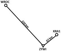
Fig. 1. Analysed baselines

2. GNSS POSITIONING

The carrier phase observations are used for technical and scientific purposes, when decimetre-or-below accuracy is demanded. To eliminate some systematic errors, phase difference observations are used. For satellite s and receiver r, a carrier phase linear observation on frequency L is defined as (Garcia, Mercader & Muravchik, 2005; Kaplan & Hegarty, 1997):

(1)

where: is the measured pseudorange between receiver r and satellite s, is the wavelength for the frequency in use, is the integer carrier phase ambiguity, is the propagation speed of the electromagnetic wave in space, is the receiver clock error, is the satellite clock error, is the initial carries phase, is the ionospheric delay, is the tropospheric delay time offset between, and is a carrier phase measurement error due to receiver noise and multipath. Single-difference (SD) observations are defined as subtraction two carrier phase observations (1) for two receivers. SD eliminates satellite clock error due to referencing to the same satellite. When two receivers are simultaneously tracking two satellites, double-difference (DD) observations can be formed as follows (Garcia et al., 2005; Li, Wu, Zhao & Tian, 2017):

(2)

where b is the reference receiver, r is the rover receiver, s is the reference satellite and q is the non‑reference satellite. Receiver clock error is eliminated by differencing between the simultaneously tracked s and q satellites. In differential positioning, DD phase observation equations are most commonly used. Linear combinations of (2) on two frequencies allow us to eliminate ionospheric delay. The so-called L3 ionosphere‑free combination (Witchayangkoon, 2000) approach is most commonly used for precise measurements.

The GLONASS system uses FDMA technology for the identification of individual satellites, thus DD observation equations can be written as follows (Dach & Walser, 2013):

(3)

where the is referred to as a SD bias term, which destroys the integer nature of DD ambiguities in Equation (3). Different frequencies and different carrier wavelengths between satellite pairs are crucial for GLONASS ambiguity resolution. The bias introduced in the DD scenario is proportional to the initialization bias of SD ambiguities and the frequency difference between pairs of satellites under consideration. Based on the above assumptions, the SIGMA strategy can be applied for the purpose of GLONASS ambiguity resolution.

Static measurements are mostly used when the most-accurate elaborations are needed, such as landslide movements (Komac, Holley, Mahapatra, van der Marel & Bavec, 2015) and crustal deformation monitoring (Rajner & Liwosz, 2011). Research shows that integrated hybrid GNSS positioning allows us to achieve accuracy that is better than GPS-only accuracy in any case (Naesset, Bjerke, Bvstedal & Ryan, 2000), or during part of a survey (Przestrzelski, Bakuła & Galas, 2016). On the other hand, as Alcay and Yigit (2016) reported, 24 h sessions and <30° elevation cut-off angles in GPS-only and GPS/GLONASS solutions produce the same results. Only for 40° cut-off angles and 4 h observation sessions do GPS/GLONASS observations improve accuracy, compared to GPS-only, although these authors did not analyse GLONASS‑only solutions (Alcay & Yigit, 2016). For daily observations, due to the current state of available software, GPS results tend to be slightly better than GLONASS results (Zheng et al., 2012). On the other hand, RTK measurements show that hybrid GNSS is slightly more accurate than GPS (Roh, Seo & Lee, 2003).

3. METHODOLOGY

The research object involved daily observations on three permanent EPN stations, i.e., ZYWI (Żywiec, Poland), KRA1 (Kraków, Poland) and WROC (Wrocław, Poland) between 1 January and 31 March (1-90 DOY). The baselines were 67 km and 220 km long, although ZYWI was a reference station whose coordinates at the observation epoch, which were obtained by the daily EPN solution, were fixed. The elaboration was made using Bernese GNSS Version 5.2 algorithms for daily observations with 30 s sampling intervals (Figure 2). The author modificated the algorithms to prepare three different scenarios: GPS, GLONAS and GNSS. Daily DD solutions were made in GPS-only, GLONASS‑only and hybrid GNSS (GPS+GLONASS) modes using precise IGS final products on frequencies L1 and L2.

Fig. 2. Diagram of processing using Bernese GNSS software

During elaboration, the ambiguity resolution strategy was quasi-ionosphere-free (QIF), while global ionosphere models obtained from IGS processing at CODE were used. The tropospheric effects were modelled using the Vienna Mapping Function (VMF1) with no estimation of the horizontal troposphere gradient, due to single baselines being processed (Dach & Walser, 2013). During data cleaning, the cut-off elevation angle was set to values presented in Table 1. Ionosphere effects were modelled applying the L3 ionosphere-free combination. Solutions were also divided into four different minimal elevation cut-off angles (Table 1).

Tab. 1

Sky visibility related to the cut-off angle

Cut-off angle	0°	3°	10°	30°	40°
Sky visibility	100%	93.4%	79.0%	44.4%	30.9%

The two biggest minimal elevation cut-off angles, 30° and 40°, cover most of the visible sky, i.e., 55% and 69%, respectively. As relative positioning was based on simultaneously tracked satellites by the rover and the reference station, the percentage number of tracked visible satellites is, in practice, always lower due to the distance between stations. Sky visibility percentages, in relation to minimal elevation cut‑off angles, is presented in Table 1. Result coordinates are subtracted from the corresponding final daily EPN coordinates at the observation epoch and transformed into a topocentric NEU frame. For statistical analysis purposes, mean absolute residuals and their standard deviations in the NEU coordinates were calculated.

Tab. 2

Mean number of visible satellites for all analysed days

Cut-off angle	3°			10°			30°			40°
System	GPS	GLO	GNSS	GPS	GLO	GNSS	GPS	GLO	GNSS	GPS	GLO	GNSS
KRA1	11.0	9.3	20.2	9.5	8.0	17.1	5.2	4.4	9.9	4.2	3.4	7.5
WROC	10.9	9.1	20.3	9.2	7.7	16.6	5.0	4.4	9.7	3.9	3.2	7.3

Table 2 presents the mean values for the number of visible satellites during the analysed 90-day period at both stations. The distance between them is 230 km, meaning that the visible constellation is very similar.

4. RESULTS

Figure 3 presents the vertical coordinate residuals for each baseline and elevation cut-off angle. In two cases, the smallest cut-off angles’ horizontal coordinates are determined with millimetre accuracy for both baselines. There are also no significant deviations between each GPS-only, GLONASS-only and GNSS solution. For 30° and 40° cut‑off angles, errors are clearly visible alongside the baseline direction, and bigger for the longer baseline (ZYWI-WROC). For those cut-off angles that slightly stand out, GLONASS-only results are the least accurate.

Figure 4 represents the residuals of the up component. The vertical component, due to the space segment construction, clock errors, tropospheric delay, multipath and antenna PCV, is two to three times less accurate than in the case of the horizontal coordinates (Yeh, Hwang, Xu, Wang & Lee, 2009). As is true for the horizontal coordinates, the most accurate are the two minimal cut-off angles, which is due to fact that the biggest number of available signals and eliminated satellites is found on the lowest elevation. Almost all residuals have a 1-2 cm accuracy. For the 30° minimal elevation cut-off angle, the up component is determined with a 3-4 cm accuracy (40°>5 cm accuracy). In each case, GLONASS‑only results are slightly less accurate, while GPS-only and GNSS results are similar to each other.

Table 3 presents the mean absolute residuals (m_N, m_E, m_U) and standard deviations (σ_N, σ_E, σ_U) of all analysed coordinate time series. For each solution (cut-off angle-related and system‑related), the smallest residuals and standard deviations are shown in bold in Table 2. For both baselines, the smaller cut‑off angle provides the better accuracy for horizontal components only. Results are strongly dependent on the length of the processed baselines, due to the number of simultaneously tracked satellites. This number decreases as the distance between stations increases.

Fig. 3. North-east residuals of analysed baselines

Fig. 4. Up component residuals of analysed baselines

Tab. 3

Mean absolute residuals and standard deviations of NEU components [mm]

Cut-off angle		3°			10°			30°			40°
System		GPS	GLO	GNSS	GPS	GLO	GNSS	GPS	GLO	GNSS	GPS	GLO	GNSS
KRA1	mN σN	1.3 1.1	1.3 1.1	1.3 1.1	1.5 1.3	1.5 1.3	1.4 1.1	2.6 2.3	2.6 2.6	2.5 2.0	4.9 3.7	4.5 4.5	4.6 3.7
	mE σE	1.3 0.8	2.2 1.8	1.3 0.8	1.5 0.9	2.4 1.6	1.5 0.9	2.1 2.5	3.6 3.8	1.8 2.2	1.4 3.7	7.5 6.1	3.7 3.5
	mU σU	10.5 4.7	11.4 5.0	10.4 4.7	6.5 4.2	7.5 4.3	6.2 4.3	8.6 7.1	8.6 6.5	8.3 7.3	17.5 11.9	14.2 14.3	14.0 12.4
WROC	mN σN	0.9 0.7	1.0 0.7	0.9 0.7	1.3 1.0	1.4 1.1	1.3 1.0	7.4 6.8	8.2 7.2	8.6 6.9	4.1 9.2	10.0 10.9	9.6 8.8
	mE σE	1.0 0.8	1.1 0.9	1.1 0.8	1.0 1.2	1.1 1.2	1.1 1.2	5.7 6.4	6.4 6.9	6.6 6.4	6.6 9.5	11.2 12.0	9.6 9.5
	mU σU	8.2 4.4	8.4 4.5	8.2 4.3	6.0 4.2	6.3 4.3	5.9 4.0	23.7 10.0	22.3 10.6	22.9 10.2	22.5 15.7	22.5 15.0	23.8 16.1

In case of the up component, this is more precisely determined for the 10° cut-off angle than for 3°. For two minimal cut‑off angles, the north and east components are calculated with a 0.7‑1.1 mm and 0.8-1.8 mm accuracy, respectively. For the up component, the accuracy is between 4.2 and 5.0 mm. There are also no significant differences between the GPS-only, GLONASS-only and GNSS results. In the case of the 30° elevation cut‑off angle, the horizontal components for each solution are two to six times worse than the 3° and 10° cut-off angles (e.g., WROC station, east component). Note that, for the three smallest elevation cut-off angles, the solutions (GPS-only, GLONASS-only and GNSS) are generally similar. For the 40° cut-off angle, the GLONASS results are the worst. Comparing the GPS and hybrid GNSS results shows that they are at the same level, while, for the ZYWI-WROC baseline, the GPS-only results are even better than those for GNSS.

5. SUMMARY

This study presented a comparison of GPS-only, GLONASS-only and hybrid GNSS solutions for 24 h observations with 30 s sampling intervals, according to the elevation cut‑off angle. The research referred to 90 consecutive observations on two baselines with relative positioning, with the use of Bernese GNSS Version 5.2 software. The resulting coordinates were compared with corresponding daily EPN solutions. This work was carried out in order to check the practical benefits of adding GLONASS signals to an existing GPS involving obstacles. For the three smallest elevation cut-off angles, there were no significant differences between each solution (GPS-only, GLONASS-only, GNSS). It was demonstrated that GLONASS-only solutions can be comparable to the others, albeit only for small elevation cut-off angles; for the greatest elevation cut-off angle, these types of solutions result in differences, especially for horizontal components. A hybrid GNSS solution also revealed insignificant benefits compared to the GPS-only approach. For each elevation cut‑off angle, GPS-only and hybrid GNSS results had the same accuracy level. GLONASS observation results were less accurate than for GPS, probably due to the algorithms used in the software. In the case of big cut-off angles, more satellites did not produce more accurate coordinates when using two GNSS systems. The results presented in this study do not validate the contributions and advantages of adding GLONASS to GPS‑only observations in obstructed sky view areas and 24 h observation sessions.

Acknowledgements

This paper was prepared within the scope of the AGH University of Science and Technology’s statutory research projects, 11.11.150.444 and 15.11.150.397.

References

1. Alcay S., C. Inal, C. Yigit, M. Yetkin. 2012. “Comparing GLONASS-only with GPS-only and hybrid positioning in various length of baselines”. Acta Geodaetica et Geophysica Hungarica 47(1): 1-12. DOI: https://doi.org/10.1556/AGeod.47.2012.1.1

2. Alcay S., C.O. Yigit. 2016. “Network based performance of GPS-only and combined GPS/GLONASS positioning under different sky view conditions”. Acta Geodaetica et Geophysica. DOI: https://doi.org/10.1007/s40328-016-0173-5.

3. Angrisano A., S. Gaglione, C. Gioia. 2013. “Performance assessment of GPS/GLONASS single point positioning in an urban environment”. Acta Geodaetica et Geophysica 48(2): 149-161. DOI: https://doi.org/10.1007/s40328-012-0010-4.

4. Cai C., Y. Gao. 2012. “Modeling and assessment of combined GPS/GLONASS precise point positioning”. GPS Solutions 17(2): 223-236. DOI: https://doi.org/10.1007/s10291-012-0273-9.

5. Charles J. 2010. An Introduction to GNSS. NovAtel Inc.

6. Dach R., P. Walser. 2013. Bernese GNSS Software Version 5.2.

7. Garcia J.G., P.I. Mercader, C.H. Muravchik. 2005. “Use of carrier phase double differences”. Latino American Applied Research 35: 115-120.

8. Guo F., X. Li, X. Zhang, J. Wang. 2017. “Assessment of precise orbit and clock products for Galileo, BeiDou, and QZSS from IGS Multi-GNSS Experiment (MGEX)”. GPS Solutions 21(1): 279-290. DOI: https://doi.org/10.1007/s10291-016-0523-3.

9. Hofmann-Wellenhof B., H. Lichtenegger, E. Wasle. 2008. GNSS – Global Navigation Satellite Systems. Vienna: Springer Vienna. DOI: https://doi.org/10.1007/978-3-211-73017-1.

10. Kaplan E., C. Hegarty. 1997. Understanding GPS. Norwood, MA: Artech House.

11. Kleusberg A. 1990. “Comparing GPS and GLONASS”. GPS World 1(6): 52-54.

12. Komac M., R. Holley, P. Mahapatra, H. van der Marel, M. Bavec. 2015. “Coupling of GPS/GNSS and radar interferometric data for a 3D surface displacement monitoring of landslides”. Landslides 12(2): 241-257. DOI: https://doi.org/10.1007/s10346-014-0482-0.

13. Li G., J. Wu, C. Zhao, Y. Tian. 2017. “Double differencing within GNSS constellations”. GPS Solutions. DOI: https://doi.org/10.1007/s10291-017-0599-4.

14. Naesset E., T. Bjerke, O. Bvstedal, L. Ryan. 2000. “Contributions of differential GPS and GLONASS observations to point accuracy under forest canopies”. Photogrammetric Engineering & Remote Sensing: 403-407.

15. Przestrzelski P., M. Bakuła, R. Galas. 2016. “The integrated use of GPS/GLONASS observations in network code differential positioning”. GPS Solutions: 1-12. DOI: https://doi.org/10.1007/s10291-016-0552-y.

16. Rajner M., T. Liwosz. 2011. “Studies of crustal deformation due to hydrological loading on GPS height estimates”. Geodesy and Cartography 60(2): 135-144. DOI: https://doi.org/10.2478/v10277-012-0012-y.

17. Roh T.H., D.J. Seo, J.C. Lee. 2003. “An accuracy analysis for horizontal alignment of road by the kinematic GPS/GLONASS combination”. KSCE Journal of Civil Engineering 7(1): 73-79. DOI: https://doi.org/10.1007/BF02841990.

18. Schmid R., M. Rothacher, D. Thaller, P. Steigenberger. 2005. “Absolute phase center corrections of satellite and receiver antennas”. GPS Solutions 9(4): 283-293. DOI: https://doi.org/10.1007/s10291-005-0134-x.

19. Söderholm S., M.Z.H. Bhuiyan, S. Thombre, L. Ruotsalainen, H. Kuusniemi. 2016. “A multi-GNSS software-defined receiver: design, implementation, and performance benefits”. Annals of Telecommunications 71(7-8): 399-410. DOI: https://doi.org/10.1007/s12243-016-0518-7.

20. Witchayangkoon B. 2000. Elements of GPS Precise Point Positioning. PhD thesis.

21. Xu G. 2003. GPS: Theory, Algorithms and Applications. Berlin, Heidelberg, New York: Springer.

22. Yeh T.K., C. Hwang, G. Xu, C.S. Wang, C.C. Lee. 2009. “Determination of global positioning system (GPS) receiver clock errors: impact on positioning accuracy”. Measurement Science and Technology 20(7): 75-105. DOI: https://doi.org/10.1088/0957-0233/20/7/075105

23. Yongjun Z. 2002. “Combined GPS/GLONASS data processing”. Geo-spatial Information Science 5(4): 32-36. DOI: https://doi.org/10.1007/BF02826472.

24. Zheng Y., G. Nie, R. Fang, Q. Yin, W. Yi, J. Liu. 2012. “Investigation of GLONASS performance in differential positioning”. Earth Science Informatics 5(3-4): 189-199. DOI: https://doi.org/10.1007/s12145-012-0108-9

Received 04.10.2017; accepted in revised form 05.01.2018

Scientific Journal of Silesian University of Technology. Series Transport is licensed under a Creative Commons Attribution 4.0 International License

---

[1] AGH University of Science and Technology, Faculty of Mining Surveying and Environmental Engineering, 30 Mickiewicza Street, 30-059 Krakow, Poland. E-mail: maciuk@agh.edu.pl.