Article
citation information:
Chládek, P., Smetanová,
D., Krile, S. On some aspects of graph theory for optimal transport among marine ports.
Scientific Journal of Silesian University
of Technology. Series Transport. 2018, 101,
37-45. ISSN: 0209-3324. DOI: https://doi.org/10.20858/sjsutst.2018.101.4.
Petr CHLÁDEK[1],
Dana SMETANOVÁ[2],
Srećko KRILE[3]
ON SOME ASPECTS OF
GRAPH THEORY FOR OPTIMAL TRANSPORT AMONG MARINE PORTS
Summary. This paper is devoted to the Travelling
Salesman Problem as applied to Czechoslovak ocean shipping companies and their
marine ports on the Black Sea. The shortest circular path around these ports is
found and discussed. Formulation of the problem accounts for the fact that
distances between the individual cities are not the same in both directions.
The consequences that arise from this situation are studied. The used
algorithms are based on graph theory and standard logistic methods. In
addition, the results are compared with the results obtained by using a minimum
spanning tree algorithm.
Keywords: Travelling Salesman Problem; graph
theory; minimum spanning tree;
marine ports
1. INTRODUCTION
The Travelling Salesman Problem (TSP) is
formulated as a task with a given set of cities and the paths between them. The
task is to find the shortest (most economical) path passing through all the
cities and returning to the starting point. The TSP is usually formulated using
concepts based on graph theory. Graph vertices represent cities, while graph
edges refer to individual paths between cities. In the traditional view, the
solution to the problem lies in finding a closed path (a circle) on a rated
(usually non-oriented) graph, cf. [1, 8]. Contrary to the classical case, our
method recognizes that distances
between individual cities are different when travelling in the opposite
direction. Such a situation is described by means of a closed path in an
oriented graph. The TSP remains a viable topic for study, cf. [2, 7, 19-20].
The Czechoslovak
Ocean Shipping (COS) company was founded in 1959. During its existence, the
company was using 28 home ports in various countries. This paper is devoted to
the Black Sea region. In this area, the business interests of the company were
realized through seven marine ports (Braila, Galati, Reni, Izmail, Constanza, Varna, Burgas) in three
countries (Bulgaria, Romania, Ukraine). There are currently other transport
companies operating in the Czech Republic that engage in ocean shipping. These
include DSV Air & Sea s.r.o., Cargo IHL - International Shipping Company,
Multitrans CZ s.r.o. and Logex Logistics, s.r.o. These companies are represented
in most of the major world ports, including former home ports of COS. For the
history of Czechoslovak maritime shipping, see, e.g., [10, 15].
In line with the TSP principles, we search for
and also compare the shortest and longest paths from Prague, through all seven
ports and back to Prague. We assume that the trip from Prague to the Black Sea
area takes place by air, the journey then continues through the individual
ports and ends after a final return flight back to Prague. Given that, among
the cities in question, only Varna and Burgas had operational international
airports at the time COS existed,
these two locations necessarily become the second and the penultimate vertices on
our graph.
2. DATA AND METHODS
For calculating and finding the shortest
path, we are going to use the road distances between the ports listed in Table
1 and the air distances from Prague to the Black Sea. The air distance from
Prague to Varna (or from Varna to Prague) is 1,279 km and the air distance from
Prague to Burgas (or from Burgas to Prague) is 1,304 km.
Table
1
Shortest distances
(in km) [7]
|
Varna |
Burgas |
Constanza |
Izmail |
Reni |
Galati |
Braila |
|
|
Varna |
- |
- |
160 |
438 |
372 |
349 |
332 |
|
Burgas |
- |
- |
290 |
502 |
436 |
414 |
393 |
|
Constanza |
158 |
288 |
- |
283 |
217 |
194 |
178 |
|
Izmail |
435 |
503 |
283 |
- |
66 |
89 |
111 |
|
Reni |
369 |
437 |
217 |
66 |
- |
23.3 |
44.4 |
|
Galati |
346 |
414 |
194 |
89 |
23.3 |
- |
21.5 |
|
Braila |
330 |
392 |
177 |
110 |
44.6 |
21.7 |
- |
We emphasize that, in most
theoretical tasks of this type, it is assumed that the distances between two
vertices A and B are the same in both directions: A-B, B-A. However, in the
case of real road traffic, these distances may be different (see Table 1). The
difference may be caused, for example, by one-way roads, highway connections
and city bypasses.
The transport problem is modelled
using a graph. All graphs represented in this article are finite, connected,
weighted and closed with oriented edges. The system of traffic routes can be
transformed into a graph in which vertices represent seaports, edges represent
transport routes and weights of edges represent the energy consumed while using
the means of transport (ship, car, airplane, train or something else) between
the respective two ports. To model this situation, we create a connected graph G=(V,E), where V is the set of n
vertices and E is the set of edges as
usual. The edges are weighted.
A Hamiltonian path is a path that
visits each vertex of the graph exactly once. A Hamiltonian cycle is a closed
path that visits each vertex exactly once (except for the vertex that is both
the start and the end, which is visited twice). A graph containing a
Hamiltonian cycle is called a Hamiltonian graph. In the language of graph
theory, the TSP requires finding a Hamiltonian cycle with the smallest sum of
the weights of the edges.
Using the mathematical software
“Maple”, the length of all circular paths (Hamiltonian cycles) was
computed. All discovered circular paths were divided into two groups. The first
group included paths beginning with Prague-Burgas nodes and ending with
Varna-Prague nodes. The second group included paths beginning with Prague-Varna
nodes and ending with Burgas-Prague nodes. The paths in each group were
examined individually and arranged in terms of length from the shortest to the
longest. From each group, the five longest and five shortest paths were
selected. It has been examined whether the five shortest paths in Group 1
correspond exactly to the five shortest paths in Group 2, except for the fact
that they run in opposite directions. The same methodology was used for the
five longest trips of each group. The conclusions are presented in Table 2-5
with a subsequent analysis of the findings.
For comparison with Hamilton cycles,
we present a minimum spanning tree (MST) and its length. Although the MST does
not solve the problem of circular paths, it has significant use in logistic
processes. A typical application of such an MST algorithm would be in searching
for the most effective way for road or train lane construction, electricity
distribution, water distribution and especially engineering networks.
The spanning tree of a connected
graph G is a subgraph G´, which connects all vertices
but does not contain any cycles [9, 14]. For the MST, we denote ![]() , where
, where ![]() and E´
represents the set of n -1 edges of
the MST, such that that
and E´
represents the set of n -1 edges of
the MST, such that that ![]() . The sum of the weights
. The sum of the weights ![]() of the edges of the MST is minimal. Thus,
for subgraph G´= (V´,E´) of the graph G, we propose
of the edges of the MST is minimal. Thus,
for subgraph G´= (V´,E´) of the graph G, we propose ![]() and the spanning tree G´ of the graph G is minimal if,
for each spanning tree G´´
of the graph G, it holds that
and the spanning tree G´ of the graph G is minimal if,
for each spanning tree G´´
of the graph G, it holds that ![]() .
.
There are several generally known
algorithms that use different ways to search for the MST, e.g., Kruskal’s
algorithm [16], Prim’s algorithm or Borůvka’s algorithm.
3. RESULTS
This chapter summarizes and interprets the
results that have been obtained from input data by mathematical methods.
For the purposes of summary, in Tables 2-5,
we use the following markings for individual ports: Bu - Burgas, V - Varna, C -
Constanza, I - Izmail, R - Reni, G - Galati, Br - Braila, P - Prague.
Two paths can be considered as mutually
equivalent if these paths pass through the ports in reverse order, e.g., the
first path in Table 2 (P-Bu-Br-I-R-G-C-V-P) and the fourth path in Table
3 (P-V-C-G-R-I-Br-Bu-P). The following tables present two sets of the
five shortest and longest paths in the direction Prague-Burgas and
Prague-Varna, including the paths equivalent to them.
Table
2
The shortest paths
in the direction Prague-Burgas
|
PATH |
DISTANCE |
EQUIVALENT PATH |
DISTANCE |
|
P-Bu-Br-I-R-G-C-V-P |
3,527.3 |
P-V-C-G-R-I-Br-Bu-P |
3,529.3 |
|
P-Bu-Br-R-I-G-C-V-P |
3,527.6 |
P-V-C-G-I-R-Br-Bu-P |
3,528.4 |
|
P-Bu-Br-G-I-R-C-V-P |
3,527.7 |
P-V-C-R-I-G-Br-Bu-P |
3,528.5 |
|
P-Bu-Br-G-R-I-C-V-P |
3,528.0 |
P-V-C-I-R-G-Br-Bu-P |
3,528.8 |
|
P-Bu-R-I-G-Br-C-V-P |
3,530.5 |
P-V-C-Br-G-I-R-Bu-P |
3,534.7 |
In the left half of Table 2, we see the
shortest paths in the direction of Prague-Burgas, while the right half shows
the equivalent paths. A similar layout for the Prague-Varna paths is found in
Table 3.
Table
3
The
shortest paths in the direction Prague-Varna
|
PATH |
DISTANCE |
EQUIVALENT PATH |
DISTANCE |
|
P-V-C-G-I-R-Br-Bu-P |
3,528.4 |
P-Bu-Br-R-I-G-C-V-P |
3,527.6 |
|
P-V-C-R-I-G-Br-Bu-P |
3,528.5 |
P-Bu-Br-G-I-R-C-V-P |
3,527.7 |
|
P-V-C-I-R-G-Br-Bu-P |
3,528.8 |
P-Bu-Br-G-R-I-C-V-P |
3,528.0 |
|
P-V-C-G-R-I-Br-Bu-P |
3,529.3 |
P-Bu-Br-I-R-G-C-V-P |
3,527.3 |
|
P-V-C-Br-I-R-G-Bu-P |
3,534.3 |
P-Bu-G-R-I-Br-C-V-P |
3,532.3 |
For the five longest paths in each direction,
Tables 4-5 are compiled in an analogous manner to the Tables 2-3. Table 4
concerns the Prague-Burgas routes.
Table
4
The
longest paths in the direction Prague-Burgas
|
PATH |
DISTANCE |
EQUIVALENT PATH |
DISTANCE |
|
P-Bu-G-C-I-Br-R-V-P |
3,998.6 |
P-V-R-Br-I-C-G-Bu-P |
4,000.4 |
|
P-Bu-G-Br-R-C-I-V-P |
3,998.1 |
P-V-I-C-R-Br-G-Bu-P |
4,001.1 |
|
P-Bu-R-C-I-Br-G-V-P |
3,997.7 |
P-V-G-Br-I-C-R-Bu-P |
4,000.5 |
|
P-Bu-I-Br-G-C-R-V-P |
3,997.7 |
P-V-R-C-G-Br-I-Bu-P |
4,000.5 |
|
P-Bu-I-Br-R-C-G-V-P |
3,997.6 |
P-V-G-C-R-Br-I-Bu-P |
4,000.4 |
Table 5 contains the longest paths
in the direction Prague-Varna. It can be noticed that the table contains a
larger number of items (paths) than the previous ones, due to the existence of
four paths of identical length in kilometres (4,001.1) in fifth place.
Table
5
The longest paths in the direction Prague-Varna
|
PATH |
DISTANCE |
EQUIVALENT PATH |
DISTANCE |
|
P-V-R-C-I-Br-G-Bu-P |
4,001.7 |
P-Bu-G-Br-I-C-R-V-P |
3,997.5 |
|
P-V-I-Br-G-C-R-Bu-P |
4,001.7 |
P-Bu-R-C-G-Br-I-V-P |
3,996.5 |
|
P-V-G-C-I-Br-R-Bu-P |
4,001.6 |
P-Bu-R-Br-I-C-G-V-P |
3,996.4 |
|
P-V-I-Br-R-C-G-Bu-P |
4,001.6 |
P-Bu-G-C-R-Br-I-V-P |
3,997.4 |
|
P-V-G-Br-R-C-I-Bu-P |
4,001.1 |
P-Bu-I-C-R-Br-G-V-P |
3,997.1 |
|
P-V-R-Br-G-C-I-Bu-P |
4,001.1 |
P-Bu-I-C-G-Br-R-V-P |
3,997.1 |
|
P-V-I-C-G-Br-R-Bu-P |
4,001.1 |
P-Bu-R-Br-G-C-I-V-P |
3,997.1 |
|
P-V-I-C-R-Br-G-Bu-P |
4,001.1 |
P-Bu-G-Br-R-C-I-V-P |
3,998.1 |
From these tables, various observations can be made, which are discussed in the next chapter. Next, Figure 1 shows the MST of the examined graph. The length of the MST is 2,012.8 km.
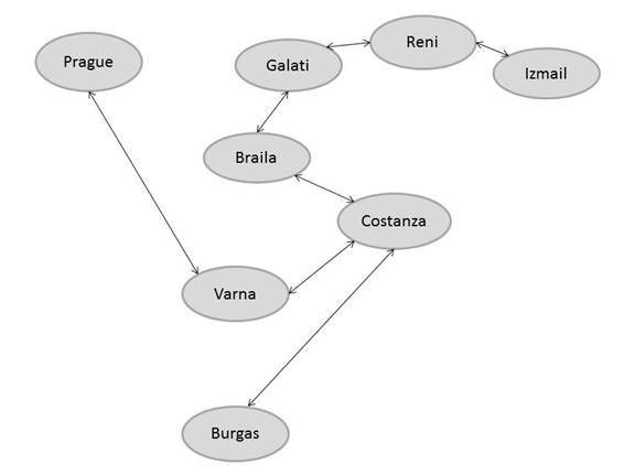
Fig. 1. MST
4. DISCUSSION
In Tables 2-5, one can see that the paths in which Varna is the second vertex are longer than the paths starting with the Prague-Burgas step.
A. Prague-Burgas direction: In this direction, the shortest path found has a length of 3,527.3 km. The cities were passed in the following order: Prague-Burgas-Braila-Izmail-Reni-Galati-Constanza-Varna-Prague (Figure 2). Due to asymmetries in Table 1, the length of this path in the opposite direction is 3,529.3 km (Table 2).
B. Prague-Varna direction: In this direction, the shortest path has a length of 3,528.4 km. The cities were passed in the following order: Prague-Varna-Constanza-Galati-Izmail-Reni-Braila-Burgas-Prague. The length of this path in the opposite direction is 3,527.6 km.
From Tables 2-3, it becomes apparent that, if we compare the five shortest paths in both directions, the following applies:
1) Of the five shortest paths in each direction, only four are mutually equivalent.
2) When arranging paths in terms of distance, the mutually equivalent paths do not appear in the same position in the order.
3) The path from Table 2, which does not have an equivalent counterpart in Table 3, and the path from Table 3, which does not have an equivalent counterpart in Table 2, both appear in fifth position in their respective tables.
4) In the direction Prague-Burgas, the distance difference between the first and the fifth path is only 3.2 km, while, in the direction Prague-Varna, it is 5.9 km. Corresponding to this fact, the distance differences in the columns displaying equivalent paths are greater in the direction Prague-Varna than in the direction Prague-Burgas.
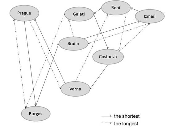
Fig. 2. The shortest and the longest Hamiltonian cycles
In a similar way, we can classify the five longest paths in both directions, as described in Tables 4-5:
1) For the direction Prague-Varna, the table contains a greater number of paths than five, because, in Table 5, there are four paths of equal length in kilometres.
2) Among the longest paths listed in both directions, there are only two equivalent ones (one in each table). Furthermore, these two paths do not appear in the same position in the order.
3) In the direction Prague-Burgas, the difference between the first and the fifth path is 1 km, while, in the direction Prague-Varna, the difference in length between the paths is only 0.6 km. Corresponding to this fact, the distance differences in the columns displaying equivalent paths are smaller in the direction Prague-Varna than in the direction Prague-Burgas.
4) The longest path of all has a length of 4,001.7 km and can be achieved in two different ways (one of them is described in Figure 2).
The overall comparison of all tables shows that the distance differences between the shortest paths are in the order of kilometres, while the differences between the longest paths are in the order of hundreds of meters.
In line with
the formulation of the problem, the Burgas-Varna edge is excluded from this
graph. This fact had to be taken into account in all calculations and also
while constructing Figures 1-2. It might appear to be more advantageous to use
the spanning tree for comparing the length of the MST and Hamiltonian cycles.
However, according to the formulation of the problem (Chapter 1), the path must
end again at the starting vertex. Therefore, when using the MST, it is
necessary to pass each edge twice (see Figure 1). Thus, the length of the path
is disproportionately increased, so it is much more advantageous to use
Hamiltonian cycles for solving this task.
5. CONCLUSION
In this paper, the discussed TSP has
an additional property, namely, that paths in opposite directions can have a
different length. The differences between the five shortest and the five
longest paths between Black Sea ports are studied and the paths are compared
with an MST. The shortest and the longest paths are found in both possible
directions. Differences between equivalent paths are discussed.
In the field of transport studies,
many different methods are being used to solve optimization problems, be it the
optimization of transport itself [2, 4, 6-7, 11-12], the placement
of logistics centres [5, 13] or the construction of transport networks
[3]. Other practical applications of a theoretical approach to freight
transport or combined transport issues are studied in [17-18, 21].
We may expect that the further study
of transport optimization will continue to take into account ever-increasing
traffic density, the increasing volume of freight transported, improvements in
technologies and rising standards of living.
Acknowledgements
This article was supported by Project Grant No.
IGS06C2 from the Faculty of Economics, University of South Bohemia, Czech
Republic.
References
1.
Applegate David L.
et al. 2006. The Traveling Salesman
Problem. Princeton: Princeton University Press. ISBN: 978-0-691-12993-8.
2.
Bartoněk
Dalibor, Jiří Bureš, Jindřich Petrucha. 2017. “Fast Herustic Algorithm Searching Hamiltonian Patrh in Graph”. 17th International Multidisciplinary
Scientific Geoconference (SGEM 2017) Conference
Proceedings - Informatics, Geoinformatics and Remote Sensing 17(21):
895-902. Sofia: STEF92 Technology Ltd.
3.
Bartuška
Ladislav, Vladislav Biba, Rudolf Kampf. 2016. “Modeling of Daily Traffic Volumes on Urban
Roads”. Proceedings of the Third
International Conference on Traffic and Transport Engineering (ICTTE):
300-304.
4.
Bartuška
Ladislav, Jiří Čejka, Zdeněk Caha. 2015. “The Application of Mathematical Methods to the
Determination of Transport Flows”. Naše
More 62(3): 91-96. ISSN: 04696255.
DOI:10.17818/NM/2015/SI1.
5.
Bartuška
Ladislav, Ondrej Stopka, Mária Chovancová et al. 2016. “Proposal of Optimizing the Transportation Flows of
Consignments in the Distribution Center”. 20th International Scientific Conference on Transport Means. Juodkrante,
Lithuania, 5-7 October 2016. Book
Series: Transport Means - Proceedings of
the International Conference: 107-111.
6.
Čejka
Jiří. 2016. “Transport Planning
Realized Through the Optimization Methods”. World Multidisciplinary Civil Engineering-Architecture-Urban Planning
Symposium 2016, WMCAUS 2016. Book Series: Procedia Engineering 161: 1187-1196.
7.
Chládek
Petr, Dana Smetanová. 2018. “Travelling Salesman Problem Applied to Black Sea Ports Used by Czech
Ocean Shipping Companies”. Naše
More. (In press.)
8.
Cook William J.
2012. In Pursuit of the Traveling
Salesman. Princeton: Princeton University Press. ISBN: 978-0-691-16352-9.
9.
Cormen Thomas H.,
Charles E. Leiserson, Ronald L. Rivest, Clifford Stein. 2001. Introduction to Algorithms, Second Edition.
MIT Press and McGraw-Hill. ISBN:0262033844 9780262033848.
10.
Herman Jan. 2015. “Czechoslovak Shipping in the Inter-war Period: The
Maritime Transport Operations of the Baťa Shoe Company, 1932-1935”. The International Journal of Maritime
History 27(1): 79-103. ISSN: 08438714. DOI: 10.1177/0843871414566579.
11.
Jelínek
Jiří. 2014. “Municipal Public
Transport Line Modelling”. Komunikacie
16 (2): 4-8. ISSN: 13354205.
12.
Jeřábek
Karel, Peter Majerčák, Tomáš Klieštik,
Katarína Valášková. 2016. “Application of Clark and Wright’s Savings
Algorithm Model to Solve Routing Problem in Supply Logistics”. Naše More 63(3): 115-119. ISSN: 04696255.
13.
Kampf Rudolf, Petr
Průša, Christopher Savage. 2011. “Systematic Location of the Public Logistic Centres
in Czech Republic”. Transport
26(4): 425-432. ISSN: 16484142. DOI: 10.3846/16484142.2011.635424.
14.
Kleinberg Jon M.,
Eva Tardos. 2006. Algorithm Design. New York: Pearson Education Inc. ISBN:
978-0321295354.
15.
Krátká
Lenka. 2016. “Czechoslovak Seafarers
Before 1989: Living on the Edge of Freedom”. The International Journal of Maritime History 28(2): 376-387. ISSN:
08438714. DOI: 10.1177/0843871416630687.
16.
Kruskal Joseph B. 1956.
“On the Shortest Spanning
Sub-tree of a Graph and the Traveling Salesman Problem”. Proceedings of the American Mathematical
Society 7: 48-50.
17.
Ližbetin
Ján, Rudolf Kampf, Karel Jeřábek et al. 2016. “Practical Application of the Comparative Analysis
of Direct Road Freight Transport and Combined Transport”. Proceedings of the 20th International
Scientific Conference Transport Means 2016. Book Series: Transport Means - Proceedings of the
International Conference: 1083-1087.
18.
Ližbetin
Ján, Ondrej Stopka. 2016. “Practical Application of the Methodology for Determining the Performance
of a Combined Transport Terminal”. Third
International Conference on Traffic and Transport Engineering (ICTTE). 24-25
November 2016, Beograd, Serbia: 382-387.
19.
Mnich Matthias,
Tobias Mömke. 2018. “Improved
Integrality Gap Upper Bounds for Traveling Salesperson Problems with Distances
One and Two”. European Journal of
Operational Research 266(2): 436-457.
20.
Pereira Armando H.,
Sebastián Urrutia. 2018. “Formulations and Algorithms for the Pickup and Delivery Traveling
Salesman Problem with Multiple Stacks”. Computers & Operations Research 93: 1-14.
21.
Stopka Ondrej,
Jozef Gašparík, Ivana Šimková. 2015. “The Methodology of the Customers’ Operation
from the Seaport Applying the ‘Simple Shuttle Problem’”. Naše More 62(4): 283-286. ISSN:
04696255.
Received 15.08.2018; accepted in revised form 21.10.2018
![]()
Scientific
Journal of Silesian University of Technology. Series Transport is licensed
under a Creative Commons Attribution 4.0 International License