Article
citation information:
Madlenak, R., Dutkova, S., Hostakova,
D., Sarkan, B. Reliability enhancement using optimization analysis. Scientific Journal of Silesian University of
Technology. Series Transport. 2018, 100,
115-125. ISSN: 0209-3324. DOI: https://doi.org/10.20858/sjsutst.2018.100.10.
Radovan MADLENAK[1],
Silvia DUTKOVA[2], Dominika HOSTAKOVA[3],
Branislav SARKAN[4]
RELIABILITY
ENHANCEMENT USING OPTIMIZATION ANALYSIS
Summary. This paper presents an
optimization analysis of a queuing system for a particular post office as a
tool to increase system reliability. The consideration of system reliability in
terms of queuing system failures is very relevant. One way to increase
reliability is to analyse the system and its parameters in order to identify
its most critical flaws. We used the chi-squared goodness-of-fit test based on
the validation of a null hypothesis over an alternative hypothesis. The purpose
of the test was to verify the correspondence of the measured data with a
theoretical probability distribution. Measurements of relevant data were
performed on the specific post office that represented the subject of our
research. This approach proved to be a powerful tool in system analysis and
optimization. The results of such an analysis can serve as the basis for the
modelling of queuing systems.
Keywords: probability
distribution; service time; chi-squared goodness-of-fit test.
1. INTRODUCTION
Each queuing system is
characterized by its parameters and attributes. A queuing system for post
offices is a stochastic system with an endless front, a certain average service
time, customer arrival input and a certain number of compartments [2,15]. In
the process of queuing system optimization, it is necessary to choose a
particular post office and analyse as accurately as possible the system
parameters. The results of this analysis cannot be generalized to each system;
therefore, the measurements only refer to the post office in question [6,10].
The system also has many random variables, which are very difficult to capture
in the system model [5,18]. However, there are several statistical tools that
can help us to determine the attributes of these random variables. The tools of
inductive statistics are used for the inductive analysis of empirical data. This
means that the results from the statistical set can be generalized to the whole
system. Discriminatory statistics, on the other hand, are only focused on a
given statistical set and the conclusions concern only those statistical units
[1].
In the case of investigating real
systems, the approach consists of a cluster of elements representing random
variables, while it is often not possible to perform measurements to obtain all
possible values of random variables. In this case, it is appropriate to use the
tools of inductive statistics to determine the sample size and generalize the
results to the entire system [17]. These results are significant for analysing
the queuing system. Such an approach allows us to optimize the system and
increase system reliability [16]. The queuing system for post offices is a
system with failures such as system overloading, inefficient system use and
overly long waiting lines. These factors not only reduce system reliability but
also increase system costs.
2. THEORETICAL BACKGROUND
While descriptive statistics have been used in various forms for several
millennia, the basics of inductive statistics, as we know and use them today,
were created in the last century. In 1908, William S. Gosset published the
article “The probable error of a mean” in Biometrics under the pseudonym “Student”. Gosset needed
statistical methods to be able to make rational decisions on the basis of a few
samples about the entire population. As a result of his efforts, we have
t-probability distribution, from which the well-known Student’s t-test is
derived [5]. The renowned statistician, Sir Ronald A. Fisher, recognized the
potential and relevance of the t-test and significantly helped to further the
development of inductive statistics. The incorrect assumption of statistics is
to consider them as only record tools. In practice, however, inductive
statistics are very important. Though tools of inductive statistics, it is
possible to analyse, for example, the sample of unemployed people who are not
interested in seeking work, and to generalize the results of the research to
the population in order to take action against unemployment. Inductive
statistics are often used by managers and economists to identify information
that can help anticipate the development of the economy, inflation and so on.
In general, indicative statistics are applicable to the investigation of
phenomena that cannot always be measured for some reason, such that research
can only be done on the basis of a representative sample. The reason for the
inability to measure all phenomena can be high measurement costs or a large
population.
There are many methods of inductive statistics, such as hypothesis
testing. The claim about one or more parameters is called the statistical
hypothesis [9]. The process in which we decide to reject or not to reject the
statistical hypothesis is called the testing of statistical hypotheses. The
process of hypothesis testing is based on the formulation of two hypotheses.
The first is a null hypothesis, which we decide to reject or not to reject. The
second hypothesis is called the alternative hypothesis, which represents the
opposite of the null hypothesis. Statistical hypotheses should be formulated so
as to be quantifiable, verifiable and statistically significant [4].
In order to know the procedure for testing statistical hypotheses, we
need to know its basic attributes (according to [11,14]):
·
feasibility (the particular test is used for a specific type of
distribution)
·
hypotheses H0, H+, level of significance α
·
test statistic
·
critical value
Some errors may occur while we are testing the hypothesis. We could
reject a null hypothesis, which should not be rejected. This error is called
a Type I error and the probability that this error occurs is called the
level of significance α. It may also transpire that we do not reject a
hypothesis, which should in fact be rejected. Such an error is called
a Type II error and the probability of occurrence of such an error is
called β. The probability of occurrence of these errors can be eliminated
by appropriate testing and a sufficient number of statistical samples [3].
There are also three types of tests.
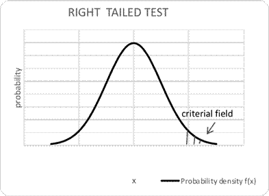
Fig. 1. Right-tailed
test of error
In the right-tailed test (Figure 1), we are also interested in the
comparison of the test statistic and the critical value. In the case where the
test statistic is greater than the critical value, we reject the null
hypothesis.
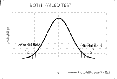
Fig. 2. Two-tailed test
of error
In the two-tailed test (Figure 2), if the test statistic is not equal to
the critical value, we reject the null hypothesis.
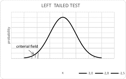
Fig. 3. Left-tailed test
of error
In the left-tailed test (Figure 3), we examine whether the calculated
test statistic is greater or less than the critical value [13]. In the case
where the value of the test statistic is less than the critical value, we
reject the null hypothesis.
3. OBJECTIVES AND
METHODOLOGY
The queuing system for post offices is a system with several parameters
and attributes. One of the parameters is the average service time. Customer
service times are continuously random variables with a certain probability
distribution. Our objective was to find out which probability distribution
belongs to the measured data in order to create a model of a queuing system for
a particular post office, which approximates to a real system. Once the model
is created, it will be possible to analyse the model, simulate it, identify its
critical points, take actions to eliminate them and thus increase the
reliability of the system.
In the first step of the research, we identified the problem of
optimizing the system and set a few subgoals, which led us to the main goal,
that is, optimizing the system.
In the second step of the research, we used an empirical method
specifically for measurement purposes. The process can be divided into three
phases:
·
a preparatory phase, which included the preparation of a paper form on
which we recorded the measured values
·
a realization phase, which included the
measurement of customer service time at a post office in Bytca with a stopwatch
·
processing phase, which included data
processing with a form suitable for further use, setting time intervals
according to a pilot measurement also performed also at the post office in
Bytca
Exact
methodology includes statistical methods, such as hypothesis testing [8]. In
order to determine the appropriate probability distribution, we used the
chi-square goodness-of-fit test to compare the observed sample distribution
with the expected probability distribution [12]. The procedure is
described in Figure 4.
The probability of a particular interval is given by
Formulas 1-2:
pi = F(bi)
. F(ai)
(1)
pi =
1 - e - λ*bi - (1 - e - λ*ai)
(2)
where:
λ is average service time
ai is the lower interval limit
bi is the upper interval limit
The test statistic is given by Formula 3:
T = ∑ (Xi - npi)2 / n*pi)
(3)
where:
Xi is the central interval value
n is the sample size
pi is the interval probability
In the last step of the research, we reached
certain conclusions about the research subject, which were based on the results
of the statistical test.
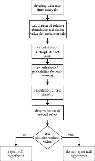
Fig.
4. Methodology of hypothesis testing
4. RESULTS
As our subgoal was to
identify and characterize average service time as a parameter of the queuing
system of a particular post office, we performed seven measurements directly at
a post office in the Slovakian town of Bytca in January 2017. The measurements
were always made at a different time during the post office’s opening
hours, so that we could capture as many as possible situations. The result of
the measurement was 700 samples, which equates to 700 customers with a certain
time of service (Table 1).
Bytca is small town with 11,000 citizens. Those measurements were made
behind a service line in cooperation with postal workers. As you can see in
Figure 5, the post office in Bytca has seven service compartments. Three of
them are universal and are therefore capable of providing most postal services.
Two of them are financial, while the last compartment is mainly for receiving
and sending parcels. All compartments were service lines in a single queuing system
and service time measurements were made arbitrarily without distinction.
Table 1
Measurement
characteristics
|
Serial number |
Place of measurement |
Date of measurement |
Time of measurement |
Tool |
Samples |
|
1 |
Post office, Bytca |
09-11-2016 |
08:00-11:30 |
Stopwatch, paper form |
60 |
|
2 |
Post office, Bytca |
11-11-2016 |
14:00-17:00 |
Stopwatch, paper form |
75 |
|
3 |
Post office, Bytca |
15-11-2016 |
12:00-16:00 |
Stopwatch, paper form |
90 |
|
4 |
Post office, Bytca |
16-11-2016 |
08:00-14:30 |
Stopwatch, paper form |
140 |
|
5 |
Post office, Bytca |
23-11-2016 |
08:00-14:00 |
Stopwatch, paper form |
125 |
|
6 |
Post office, Bytca |
25-11-2016 |
13:00-17:00 |
Stopwatch, paper form |
100 |
|
7 |
Post office, Bytca |
29-11-2016 |
08:00-13:00 |
Stopwatch, paper form |
110 |
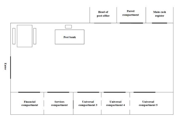
Fig. 5. Layout of post office in Bytca
The subject of measurements concerned customer service times. The
customers of the post office came with various requirements, which affect the
length of service time. It is very important to understand that service time is
not the time that a customer spends in a transaction. We stop the stopwatch
after the post worker finish the last activity associated with the service. The
service time depends on the type of service that a customer requests, the
number of requests and failures of information system or technology equipment.
The length of the service time is also affected by the worker‘s service
speed. These factors can be reflected in average service time. In the next
step, measured data were divided to time intervals.
Table 2
Statistical characteristics of measurement in the post office in Bytca
|
Class i |
Class interval |
Central interval |
Absolute frequency |
Relative frequency in% |
Cumulative absolute
frequency |
Cumulative relative
frequency in% |
|
1 |
(0,2> |
1 |
301 |
43 |
301 |
43 |
|
2 |
(2,4> |
3 |
184 |
26 |
485 |
69 |
|
3 |
(4,6> |
5 |
98 |
14 |
583 |
83 |
|
4 |
(6,8> |
7 |
59 |
8 |
642 |
92 |
|
5 |
(8,10> |
9 |
36 |
5 |
678 |
97 |
|
6 |
(10,∞> |
11 |
22 |
3 |
700 |
100 |
In the order to determine which probability distribution is going to be
tested, we plotted a histogram, which showed that it could be an exponential
distribution. In fact, the service times in queuing systems generally fit to
exponential distribution. So, we decided to use the chi-squared goodness-of-fit
test to test data for exponential distribution. As this is a single-tailed
test, we did not have to choose the type of test.
4.1. Chi-squared goodness-of-fit
test
Null hypothesis H0 means that the service
time is modelled according to exponential distribution; while alternative
hypothesis H1 means that the service time is not modelled
by exponential distribution. The level of significance reflects the probability
that we reject the true hypothesis. In general, this probability must be low
and therefore we have chosen 
The objective of the chi-squared goodness-of-fit test is to compare the
calculated test statistic and the critical value, which can be found in the
chi-square distribution table. The calculation of the test statistic is given
by the mathematical relationship according to Formula 3, where pi represents
the probabilities of individual class intervals. These probabilities can be
calculated using Formulas 1-2, where α and β are class interval
boundaries, and parameter ![]() is
is ![]() average service time. In Table 3,
we can observe the probability classes with test criteria values for each class
interval.
average service time. In Table 3,
we can observe the probability classes with test criteria values for each class
interval.
After calculating the
test statistic, we took the critical value χ2 - the distribution
corresponding to the chosen significance level and the degree of freedom f:
χ2 0.05(7-1-1)=χ2 0.05(5)=11.0705 (3)
If the test statistic is less than the critical value, we do not reject the
null hypothesis:
T<χ20.05
(4)
10.6778<11.0705
As the test statistic is not greater than the critical value, we do not
reject the null hypothesis. This means that the service times at the post
office in Bytca fit to exponential distribution (Figure 6).
Table 3
Probability classes with
test criteria values for each class interval
|
Class i |
(ai,bi> |
xi |
ni |
xi*ni |
pi |
Ti |
|
1 |
(0,2> |
1 |
313 |
313 |
0.4615 |
0.3116 |
|
2 |
(2,4> |
3 |
187 |
561 |
0.2485 |
0.9773 |
|
3 |
(4,6> |
5 |
94 |
470 |
0.1338 |
0.0011 |
|
4 |
(6,8> |
7 |
49 |
343 |
0.0721 |
0.0417 |
|
5 |
(8,10> |
9 |
32 |
288 |
0.0388 |
0.8591 |
|
6 |
(10,12> |
11 |
19 |
209 |
0.0209 |
1.3046 |
|
7 |
(12,∞) |
13 |
6 |
78 |
0.0244 |
7.1824 |
|
∑ |
700 |
2,262 |
10.6778 |
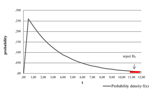
Fig. 6. Chi-squared goodness-of-fit test:
exponential distribution of time service at the post office
5. CONCLUSION
By using the inductive
statistics tool, we have found that random variable service time at a
particular post office fits with exponential distribution. Service times in
systems such as queuing systems in post offices fit to exponential distribution
in most cases. This means that the probability of service time t+x is less than the probability of
service time t, and decreases exponentially. This discovery has helped us in
the process of building a model of a queuing system for a particular post
office. Our samples, which are generated by a random function in the post
office queuing system model, are from a uniform distribution (0,1). However,
the random variables in real systems including service times do not fit to
uniform distribution, such that it is necessary to determine the appropriate
probability distribution. In the next step, we transformed uniform distribution
samples into samples that fit to probability distribution by a given algorithm.
The process of building a queuing model is one of the most important steps in
system optimization.
Analysing system
attributes and applying them correctly in a model are important in order to
achieve the most accurate results. This model is applicable to all analogical
queuing systems, but it is necessary to measure the input parameters of service
time and customer input for a particular post office, as well as take into
consideration different attributes of the post office, such as the number of
compartments and the range of services. The reliability of a system reflects
its performance and the satisfaction of customers, especially in queuing
systems where customers want to be served. One of our optimization goals was to
increase system reliability by optimizing the number of service compartments at
individual time intervals, which ultimately led to a reduction in customer
queues and customer waiting times. Such optimization can also result in
maintenance cost reduction and an overall increase in system efficiency. It can
also serve as a starting point in the compilation of post office staffing
schedules.
Acknowledgements
This paper was supported
by the scientific grant VEGA 1/0721/18 for research on the economic
impacts of visual smog on transport using methods of neuroscience.
References
1.
Achimska V. 2011. Modelovanie
systemov. [In Slovak: System
Modelling.] Zilina: Zilinska univerzita v Ziline. ISBN
978-80-554-0450-9.
2.
Droździel P., B. Bukova, E. Brumercikova. 2015. “Prospects
of international freight transport in the East-West direction”. Transport
Problems 4(10): 5-13.
3.
Galambos J., S. Kotz. 1978. Characterizations
of Probability Distributions. New York: Springer. ISBN 3-540-08933.
4.
Good P.I., J.W. Hardin. 2009. Common
Errors in Statistics (and How to Avoid Them). Hoboken, NJ: Wiley &
Sons.
5.
Husek, R. J. Lauber. 1987. Simulacne
modely. [In Czech: Simulation Models.]
Prague: ALFA. ISBN 04-326-87.
6.
Kolarovszki P., J. Tengler, M. Majercakova. 2016. “The new model
of customer segmentation in postal enterprises”. In Third International Conference on New Challenges in Management and
Business: Organization and Leadership 230: 121-127.
7.
Lehmann E.L. ‘Student‘ and small sample theory”. Statistical
Science 14(4): 41-426.
8.
Lyocsa S., Baumohl E., Výrost T. 2013. Kvantitativne metody v ekonomii II. [In Slovak: Quantitative Methods in Economics II.] Košice: Elfa. ISBN 978-80-8086-210-7.
9.
Montgomery D.C., G.C. Runger. Applied
Statistics and Probability for Engineers. New York, NY: John Wiley &
Sons.
10.
Matuskova M., L. Madlenakova. 2016. “The impact of the electronic
services to the universal postal services”. In Proceedings of the 16th International Scientific Conference Reliability
and Statistics in Transportation and Communication (Relstat-2016) 178: 258-266.
11.
Mrkvicka T., V. Petraskova. 2006. Uvod
do statistiky. [In Czech: Statistics
Introduction.] Ceske Budejovice: Jihočeská univerzita. ISBN
80-7040-894-4.
12.
Plackett R., L. Pearson. 1983. “The chi-squared test”. International Statistical Review 51:
59-72.
13.
Rui H., C. Hengjian. 2015. “Consistency of chi-squared test with
varying number of classes”. Journal
of System Sciences and Complexity 28: 439-450.
14.
Tkac M. 2001. Statisticke riadenie
kvality v praxi. [In Slovak: Statistical
Quality Management in Practice.] Bratislava: Ekonom.
15.
Xing Y.A., D.B. Grant, A.C. McKinnon, J. Fernie. “Physical
distribution service quality in online retailing”. International Journal of Physical Distribution & Logistics
Management 40(5-6): 415-432.
16.
Yi C.G., S.D. Ju. 2006. “Service reliability analysis on logistics
network”. Proceedings of the IEEE
International Conference on Service Operations and Logistics, and Informatics
(Soli 2006).
17.
Zo H., D.L. Nazareth, H.K. Jain. 2012. “End-to-end reliability of
service oriented applications”. Information
Systems Frontiers 14(5): 971-986.
18.
David Shteinman2014. “Two methods to improve the
quality and reliability of calibrating and validating simulation models”.
Road & Transport Research: A Journal
of Australian and New Zealand Research and Practice 23(3). ISSN: 1037-5783.
Received 02.03.2018; accepted in revised form 16.08.2018
![]()
Scientific
Journal of Silesian University of Technology. Series Transport is licensed
under a Creative Commons Attribution 4.0 International License