Hristina
GEORGIEVA, Lilo KUNCHEV[1]
VEHICLE TRAJECTORY MODELING UNDER THE INFLUENCE
OF LATERAL SLIDING
Summary. This paper presents an analysis of
vehicle trajectory on curved path, in the presence of lateral sliding. The pure
rolling motion is not always possible especially where working conditions are
rough and not predictable. To take sliding effects into account, the variables
which characterize sliding effects are introduced into the mathematical model
(steering angle, vehicle speed, tire cornering stiffness and etc.). This
mathematical model is linear with two freedom degrees. From the study based on
the verification of force in the contact zone tire/ground, we conclude that
speed exceeding 60 km/h and small steering angles can destabilize the vehicle.
Keywords: Steering
angle, vehicle speed, tire cornering stiffness, vehicle trajectory
Modelowanie trajektorii pojazdu pod wpływem przesunięcia bocznego
Streszczenie. W artykule przedstawiono analizę trajektorii ruchu pojazdu na zakrzywionym
torze, w obecności przesunięcia bocznego. Czysty ruch toczny nie jest zawsze
możliwy, zwłaszcza gdy warunki pracy są niebezpieczne i nie do przewidzenia. By
wziąć pod uwagę zmienne efekty przesuwne, charakteryzujące działanie przesuwne,
do modelu matematycznego są wprowadzone kąt kierownicy, prędkość pojazdu,
sztywność opon na zakrętach itp. Ten model matematyczny jest liniowy o dwóch
stopniach swobody. Z badań opierających się na weryfikacji obowiązujących w
strefie styku opony/ziemia, możemy stwierdzić, że prędkość przekraczająca 60
km/h oraz małe kąty skrętu mogą zdestabilizować ruch pojazdu.
Słowa kluczowe:
Kąt skrętu, prędkość pojazdu, sztywność opon, trajektoria ruchu
pojazdu
1. INTRODUCTION
The behavior of the vehicles represents the
results of the interactions among the driver, the vehicle and the environment.
The problem of vehicle motion on a curved path represents
a subject of high interest and it is important part of vehicle safety. The
motion is influenced by many external factors such as road roughness, lateral
aerodynamics, and tire construction
[2, 5, 7]. Examination of the vehicle trajectory needs all this factors to be
evaluated. With the development of the electronics and mechatronics applied in
the automotive industry there are always new solutions how to keep the vehicle
stable and how to control the vehicle trajectory.
For the vehicle
safety, one of the most complex components is the tire and the road interaction
problem. While moving in a curve, forces appear at the contact surfaces between
the wheel and the road. Under these forces, the tires are deformed and the
velocity on the wheel is deviated from the wheel plane under a certain angle,
depending on the tire lateral rigidity and force magnitude (see Fig. 1).
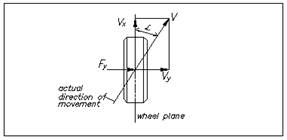
Fig. 1. Tire slip angle
Rys. 1. Kąt poślizgu opony
The tire plays
an important role in the performance of the vehicle model. The modeling of
vehicle dynamic behavior has to take into account the tire elastic in the
contact zone tire/road (see Fig. 2). This will give the possibility of better
predict and control of the vehicle trajectories. More or less complicated
variants of the tire model can be found in literature
[3, 5].
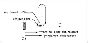
Fig. 2. Contact zone tire/road
Rys. 2. Miejsce kontaktu opony z drogą
The
movement on a curved trajectory has been treated in numerous papers [1, 3, 6, 9,
10]. In general, these authors use the fundamental principles of dynamics. For
example, to describe the lateral dynamics, Segal [10] presents a vehicle model
with three degrees of
freedom in order to describe lateral movements. If roll movement is ignored, a
simple model known as the “Bicycle Model”
is obtained. This model is currently used for studies of lateral vehicle
dynamics (yaw, lateral speed and slip angle).
This paper
is consecrated of the vehicle movement on curved trajectory using a model of
two degree of freedom. The main objective is to study the influence of some
vehicle properties such as vehicle speed, position of vehicle center of
gravity, tire cornering stiffness and steering angle while the vehicle is
turning. In this context, a mathematical-mechanical model is developed to
describe the vehicle behavior in large interval of driving conditions from
normal to the limits of controllability. This model has two degrees of freedom
(df): translation around the axis Oy and rotation in axis Oz.
The complete vehicle is considered as suspended mass related to the wheels.
This simple model is currently used in the literature to describe the lateral
acceleration, yaw and slip angle. In fact, these parameters permit to describe
a vehicle during the turning maneuver. The study aims is to define the criteria
for the detection of critical situations.
The paper is
structured as follows: Section 1
provides introductive elements, notations and motivations. Section 2 introduces the linear vehicle model, used for the
simulation. Section 3 describes the
simulation method and the indicator proposed to determine
the risk of tire lateral slipping. In Section
4, the results are analyzed and shown that the vehicle speed is the most
critical for vehicle stability while cornering. Conclusions and discussions are
given in Section 5.
2. THE MATHEMATICAL MODEL
Modeling
the vehicle dynamic behavior in all is a complex subject and requires good
knowledge of the components involved and their physics [1,2]. The first step in
the study of the vehicle lateral behavior is to create a mathematical model
that have to represent the physical system with good approximation. The
formulation of the following model takes into account these assumptions:
-
The vehicle and his model are symmetrical to the axis Ox;
-
The dynamical process (displacement around to the axis Oz)
isn’t exanimated;
-
The laterals forces are due of centrifuge force;
-
The tire lateral force varies linearly with the slip
angle;
-
The camber angle is neglected;
-
The tire angles (τ) are small (cos τ =1et sin τ = τ).
Fig. 3
shows the vehicle model used in this research. The vehicle model in Fig. 3 has
two degrees of freedom. The vehicle motion is defined by its translation around
the axis Oy and its rotation in the axis Oz. The vehicle
is considered as a rigid body (sprung mass) related to the wheels. This model
is completed with a linear model of force in the contact zone tire/road [7].
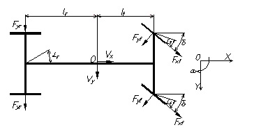
Fig. 3. „Four wheels model”
Rys. 3. „Model czterech kół”
In this
research, we have assumed the front and rear lateral forces to be
proportional to the tire slips angles. This functional link
is expressed into the following relation:
![]() (1)
(1)
The following
equations define the slip angles of front and rear tires:
 (2)
(2)
Where Cα
represents the tire cornering stiffness witch depends on road adherence µ, on
the tire internal pressure p and the tire vertical force Fz. This
parameter is essential in the evaluation of the potential of tire used [8,
11].
Finally, we
obtain a linear model with four varying parameters:
-
The longitudinal speed (V);
-
The steering angle (δ);
-
The rigidity of the tire (Cα);
-
The position of vehicles center of gravity (lf
and lr).
For the
differentials equations describing the system are valid:
![]() (3)
(3)
![]() (4)
(4)
Fig. 4 shows the block
diagram of modeling.
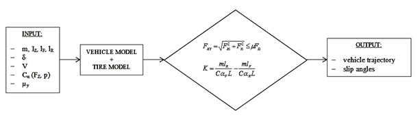
Fig. 4. Blog diagram for simulation
Rys. 4. Diagram symulacji
The block "Input" supplies the necessary
simulation data. The parameters: m, Iz, lf and lr
characterize the chosen vehicle. The steering angle δ simulates the driver
actions, while the tire cornering stiffness is chosen as a function of the tire
vertical load Fz and the tire internal pressure p.
The block "Vehicle Model+ Tire Model" uses the
data from the first block to solve differential equations 3 and 4 to obtain
lateral acceleration, yaw rate and slip angle.
The third block evaluates the vehicle
dynamic state and detects the critical situation – the saturation limit of the
efforts in the contact zone tire/road.
Finally, the
block "Output" shows the
vehicles trajectory and tires slip angles. At the same time, it indicates if
the tires are sliding and as a consequence if the limit of controllability is
achieved.
3. SIMULATION
Vehicle
model was built in MATLAB in order to analyze the state and predict the vehicle
behavior under the different initials conditions of vehicle speed, steering
angel, tire cornering stiffness and vehicles position of center of gravity.
Lateral
instability may result from slippery road conditions or excessive speed in a
curve. The poor-handling is another reason for lateral instability and which
represents a significant proportion of the vehicle accidents. In this context
and to judge the vehicles behavior while cornering is adopted a test called
"Angular dynamic". The aim
of this test is to keep the vehicle at a constant speed on a constant
radius turn with a constant steering angle [2]. This
steering behavior of the vehicle is estimated with the gradient K:
![]() (5)
(5)
Three different
steady-states can be identified:
![]() the vehicle is neutral;
the vehicle is neutral;
![]() the vehicle shows understeer;
the vehicle shows understeer;
![]() the vehicle shows oversteer.
the vehicle shows oversteer.
Equation 5 shows
the importance of the vehicle position of the center of gravity lf/lr
and tire cornering stiffness Cα in terms of maneuverability.
In this work, we
are used a pneumatic tire type "175/70R13
T 82" with internal pressure of 2 bar and variation of tire vertical
load Fz from 3 kN to 8 kN. Table 1 shows the parameters used for the
vehicles simulation. These values come from commercial specifications from
a standard European vehicle.
Table 1
Vehicle
characteristics and numerical parameters
|
№ |
Parameter |
Symbol |
Value |
|
1. |
Total masse of vehicle [kg] |
m |
1603 |
|
2. |
Total yaw inertia of vehicle [kgm2] |
Jz |
3156 |
|
3. |
Distance between CG and front axle [m] |
lf |
1,050 |
|
4. |
Distance between CG and rear axle [m] |
lr |
1,525 |
|
5. |
Tire front cornering stiffness [kN/rad] |
CαF |
(30÷50) |
|
6. |
Tire rear cornering stiffness [kN/rad] |
CαR |
(30÷50) |
|
7. |
Front steering angle [grad] |
δ |
(0-32) |
4. CASE STUDY
The figures
presented in this section show the trajectories obtained for different initial
conditions of the system. The effects of the vehicle speed, the position of
vehicle center of gravity, the tire cornering stiffness and the steering angle
are studied.
4.1.
Vehicles center of gravity is located near to the front axle
When the vehicles center of gravity is located
near to the front axle, the vehicle shows understeer (K>0), it means that the
slip angle of the front tires is greater than the slip angle of the rear
tires. Fig. 4 presents the
vehicles simulated trajectories for a vehicles speed of 5 m/s. The steering angle has been varied between 5°
and 30° and
the curves are plotted for different coefficients
of tire cornering stiffness. It can be seen from these figures that the augmentation
of the steering angle decreases the radius of
the trajectory curve. This represents a risk when the slip angles are high. Also, we can
observe that the slip angle decrease with augmentation of
tire cornering stiffness.
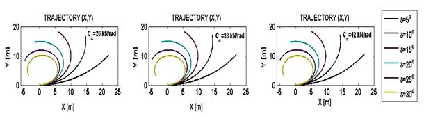
Fig. 5. Vehicle trajectory estimated for speed V = 5
m/s, K > 0, pure motion
Rys. 5. Trajektoria ruchu pojazdu dla
prędkości V = 5 m/s, K > 0, czysty ruch
In a second simulation, the vehicles speed is increased to 10 m/s. The
objective is to estimate the effect of speed on the vehicle path. The results
obtained are present in Fig. 6. By comparison with Fig. 5, it can be seen that
the displacement is increased as a consequence of the augmentation of vehicles
speed. Also, the augmentation of vehicle speed doesn’t permit to attack the
turn with steering angle greater than 10°.
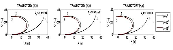
Fig. 6. Vehicle trajectory estimated for speed V = 10
m/s, K > 0
1 – motion without sliding; 2 – motion + sliding; 3 – pure sliding
Rys. 6. Trajektoria ruchu pojazdu dla
prędkości V = 10 m/s, K > 0,
1 – ruch bez poślizgu; 2 – ruch +
poślizg; 3 – czysty poślizg
When the vehicle speed
is increased to
15 m/s as can be seen from Fig. 6, the
displacement are increased too and
confirming the previous conclusions concerning the
effect of vehicles speed. At this speed,
the maximum steering angle allowed is 5°. We can
conclude that the vehicle speed controls the maximum steering angle with witch a turn can
be taken.
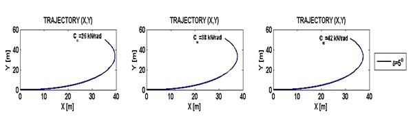
Fig. 7. Vehicle trajectory estimated for speed V = 15
m/s, K > 0, pure sliding
Rys. 7. Trajektoria ruchu pojazdu dla
prędkości V = 15 m/s, K > 0, czysty poślizg
4.2. Vehicles center of
gravity is located near to the rear axle
When the vehicles center of gravity is located
near to the rear axle, the vehicle shows oversteer (K<0), it means that the
slip angle of the rear tires is greater than the slip angle of the front
tires. Here the effect of vehicle speed gives a very large influence
because the vehicle is oversteer and the effects are much more severe.
Fig. 8 presents the vehicle simulated trajectories for
a vehicles speed of 5 m/s. The
steering angle has been varied between
5° and 30°
and the curves
are plotted for different coefficients of tire cornering stiffness, again. The steering
angles effect on the curve radius is confirmed.
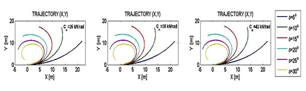
Fig. 8. Vehicle trajectory estimated for speed V = 5
m/s, K < 0, pure motion
Rys. 8. Trajektoria ruchu pojazdu dla
prędkości V = 5 m/s, K < 0, czysty ruch
Fig. 9 shows the
trajectories when the speed is augmented to 10 m/s. Once again, the vehicle
displacement increases with the augmentation of vehicle speed and the turn may
be attacked with a maximal steering angle of 10°.
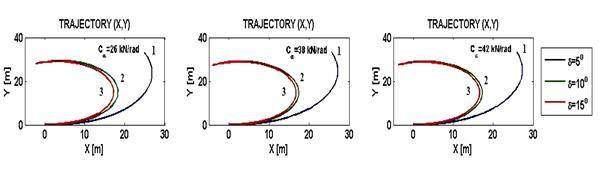
Fig. 9. Vehicle trajectory estimated for speed V = 10
m/s, K < 0
1 – motion without sliding; 2 –
motion + sliding; 3 – pure sliding
Rys. 9. Trajektoria ruchu pojazdu dla
prędkości V = 10 m/s, K < 0,
1 – ruch bez poślizgu; 2 – ruch +
poślizg; 3 – czysty poślizg
When vehicle
speed is increased to 15 m/s as can be seen from Fig. 10, the displacement are
increased too and confirming the previous conclusions concerning the effect of
vehicles speed. At this speed, the maximum steering angle allowed is 5°. We can
conclude that the vehicle speed controls the maximum steering angle with witch
a turn can be taken.
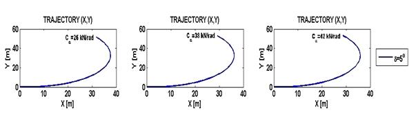
Fig. 10. Vehicle trajectory estimated for speed
V = 15 m/s, K <0, pure sliding
Rys. 10. Trajektoria ruchu pojazdu dla
prędkości V = 15 m/s, K < 0, czysty poślizg
4.3. The center of gravity is in the middle of
the vehicle
To
illustrate the influence of the tires cornering stiffness of the vehicles trajectory
we fix the center of gravity in the middle of the vehicle. Some of simulations
results are shown in Fig. 11. In this case, the simulation
is made for vehicles speed of 10 m/s and steering angles from 5o
to 10o. When the tire cornering stiffness of
front axis Cαf is
greater than the tire cornering stiffness of rear axis Cαr the vehicle has the tendency to entre too in
the turning. This means that the
slip angle of the rear tires is greater than the slip angle of the front
tires.
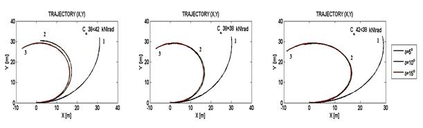
Fig. 11. Vehicle trajectory estimated for
speed V = 10 m/s, K > 0, K = 0, K < 0;
1 – motion without sliding; 2 – motion + sliding; 3 – pure sliding
Rys. 11. Trajektoria ruchu pojazdu dla
prędkości V = 10 m/s, K > 0, K = 0, K < 0,
1 – ruch bez poślizgu; 2 – ruch +
poślizg; 3 – czysty poślizg
The
conclusion that can be drawn from this study is that for speeds which exceed
60 km/h, relatively small steering angles can destabilize the vehicle in his
movement on
a curved path. Also, for steering angles greater than 10 the vehicle speed has
to decrease under 60 km/h in order to maintain a stable course.
5. CONCLUSION
One of the
objectives of this work has been to develop vehicle model that could be used to
investigate the vehicle lateral behavior. The dynamics for the vehicle have
been presented with assumptions. The purpose of this model is to characterize
the vehicle stability during the cornering follow the dynamic state of the
system and steering angle applied to the wheel.
A method is proposed to determine the risk of tire lateral slipping. The choice of
this indicator is based on the efforts estimation of in the contact zone tire /
road. This choice is justified by the fact that the saturation of efforts in
the contact zone shows that the wheel is no longer able to ensure the stability
of the vehicle.
The analysis of
the results shows that the vehicle speed has an important influence on the
vehicle stability. This can be explained by the fact that the steer angle
needed to follow a circular turn depends largely on the vehicle speed. When the
vehicle speed is increased, the tire transversals reactions rise and therefore
the slip angles also increase. The results show that the coefficient of
under/oversteer K is related to the location of the center of mass and the
stiffness value of the tire. The start of sliding isn’t at the same time for
each wheel.
Future work will
be to improve vehicle stability by implementing load transfers during the
turning maneuver [2-4].
Bibliography
1.
Genta. 1997. Motor
vehicle dynamics: modelling and simulation. Singapore: Word scientific
publishing.
2.
Gillespie T. 1992. Fundamentals
of vehicle dynamics. Warrendale PA USA: Society of Automotive Engineers
(SAE) International.
3.
Kiencke U., N. Nielsen. 2005.
Automotive control systems for engine, driveline, and vehicle. 2nd
edition. Berlin: Springer.
4.
Milliken W., D. Milliken. 1995.
Race car and vehicle dynamics. SAE International.
5.
Pacejka H.B. 2002. Tyre
and vehicle dynamics. Butterworth-Heinemann Ltd.
6.
Rajamani R. 2005. Vehicle
Dynamics Control. Berlin: Springer.
7.
Wong J. 1978. Theory of
ground vehicles. New York: John Wiley and Sons, Inc.
8.
Танева Ст. 2013. “Изследване на напречното увличане на пневматична гума”. [Taneva St. 2013. “Izsledvane na
naprechnoto uvlichane na pnevmatichna guma”]. [In Bulgarian: “Research on
cross-entrainment of the tire”]. Journal of the Technical University –
Sofia. Plovdiv branch 19.
9.
Niculescu-Faida O., S. Iliescu,
I. Făgăraşan, A. Niculescu-Faida. 2008. “Vehicle stability study on curved
trajectory”. Buletinul Ştiinţific U.P.B., Seria C – Inginerie Electrică
70(2).
10.
Segal M. 1956. “Theoretical
prediction and experimental substantiation of the response of the automobile
to steering control”. Proc. Automobile division of the institute of
mechanical engineers 7.
11.
Иванов Р. Изследване коефициента на напречно увличане на пневматични гуми за леки автомобили. Русе,
НТ на РУ`2011, том 50, серия 4. [Ivanov R. Izsledvane koeficienta na naprechno
uvlichane na pnevmatichni gumi za leki avtomobili. Ruse, NT na RU`2011, tom 50, serija 4]. [In Russian: Study
coefficient of cross-entrainment of tires for cars].
Nomenclature:
m – total masse of
vehicle, kg,
Iz – total
yaw inertia of vehicle, kgm2,
Vx –
vehicle speed around Ox, m\s ,
lf & lr
– distance between CG and front & rear axle, m,
Cαf & Cαr – tire
front & rear cornering stiffness, N/rad,
δ – steer front angle,
αf & αr – front & rear tire slip angle, degree,
y – displacement
around lateral axis Oy, m,
ψ – yaw motion (rotation in axis Oz), degree,
Fxn –
representing the longitudinal efforts in the contact zone tire/road, N,
Fyn –
representing the lateral efforts in the contact zone tire/road, N,
![]() – lateral
acceleration, m/s2,
– lateral
acceleration, m/s2,
![]() – yaw
acceleration, rad/s2,
– yaw
acceleration, rad/s2,
K – coefficient understeer
or oversteer.